The BEAM Book
Written by Erik Stenman and contributors.
This work is licensed under a Creative Commons Attribution 4.0 International License (CC BY 4.0). This means you are free to share, copy, redistribute, and modify this book under the following terms:
-
Attribution: Credit must be given to the original authors and contributors.
-
No Additional Restrictions: You cannot impose legal restrictions that prevent others from using the book freely under the same terms.
Contributors: Special thanks to Richard Carlsson, Yoshihiro Tanaka, Roberto Aloi and Dmytro Lytovchenko.
For full attribution details, visit: https://github.com/happi/theBeamBook/graphs/contributors.
Free Digital Version Available. This book is freely available online at https://github.com/happi/theBeamBook/ under the Creative Commons license. This printed edition is provided for convenience.
For more information on the Creative Commons license, visit: https://creativecommons.org/licenses/by/4.0/.
First Edition, 2025 ISBN: 978-91-531-4253-9
© 2025 Erik Stenman.
- Preface
- I: Understanding ERTS
- 1. Introducing the Erlang Runtime System
- 2. The Compiler
- 3. Processes
- 4. The Erlang Type System and Tags
- 5. The Erlang Virtual Machine: BEAM
- 6. Modules and The BEAM File Format
- 7. Generic BEAM Instructions
- 8. Different Types of Calls, Linking and Hot Code Loading
- 9. The BEAM Loader
- 10. Scheduling
- 11. The Memory Subsystem: Stacks, Heaps and Allocators
- 11.1. The Memory Subsystem
- 11.2. Different Types of Memory Allocators
- 11.3. Per-Scheduler Allocator Instances
- 11.4. System Flags for Memory
- 11.5. Commonly Used Flags
- 11.6. Special Flags for
mseg_alloc - 11.7. Special Flags for
sys_alloc - 11.8. Literal Allocator (
literal_alloc) - 11.9. Global and Convenience Flags
- 11.10. Practical Examples
- 11.11. Recommendations
- 11.12. Process Memory
- 11.13. Other Interesting Memory Areas
- 12. Garbage Collection
- 13. IO, Ports and Networking
- 14. Distribution
- 15. How the Erlang Distribution Works
- 16. Interfacing Other Languages and Extending BEAM and ERTS
- II: Running ERTS
- Appendix A: Building the Erlang Runtime System
- Appendix B: BEAM Instructions
- Appendix C: Full Code Listings
- References
Preface
Erlang and Elixir runs on one of the most robust virtual machines ever built. This book shows you how it works, not only conceptually, but at the level where things actually happen.
This book is not a style guide. It’s not about syntax or best practices. It won’t teach you how to structure your GenServers or argue about supervision trees.
What it will do is walk you through the internals of the BEAM. How it schedules processes. How it allocates memory. How it handles concurrency. How it makes trade-offs under pressure. The things that matter when your system is live, and bugs don’t show up in tests.
Toward the end, we’ll get into tracing, profiling, and performance tuning. But the real goal is to give you the tools to understand what your code is doing at runtime, and why.
When you know how the system behaves, you can stop guessing.
About this book
This book is for you if:
-
You want to understand how Erlang really works.
-
You want to tune a BEAM installation for performance or reliability.
-
You want to debug crashes and strange behavior inside the VM.
-
You want to get the most out of your systems in production.
-
Or maybe you just want to build your own runtime, from the ground up.
If you’re only here for performance tricks, feel free to skip ahead to the later chapters. But if you want to understand what’s going on beneath those tools, how the system actually works, start from the beginning.
The deeper your understanding, the better your decisions.
Conventions Used in This Book
The BEAM VM can run on a wide range of systems, from small embedded hardware to large multi-core servers with terabytes of memory. To optimize the performance of BEAM applications effectively, you must understand how the VM utilizes memory and other resources.
Throughout this book, we use diagrams extensively to explain memory structures and data layouts clearly. Because memory layouts and stack operations can vary in their representation, here are the conventions we’ve adopted for diagrams:
-
Memory Diagrams:
-
Memory addresses increase upwards in our diagrams.
-
Low memory addresses appear at the bottom; high addresses at the top.
-
Stacks typically grow downward, starting at higher addresses, with new elements pushed onto lower addresses.
-
-
C-Structure Diagrams:
-
C-structures are represented with their first fields at the top, even though these first fields occupy lower memory addresses.
-
This results in diagrams of structures appearing inverted relative to general memory-area diagrams.
-
Be aware that when structures and memory areas appear together in diagrams, their address representations will be mirrored. Understanding this convention will help prevent confusion when interpreting visual examples throughout the book.
You don’t need to be an Erlang programmer to read this book, but you will need some basic understanding of what Erlang is. This following section will give you some Erlang background.
Erlang
In this section, we will look at some basic Erlang concepts that are vital to understanding the rest of the book.
Erlang has been called, especially by one of Erlang’s creators, Joe Armstrong, a concurrency oriented language. Concurrency is definitely at the heart of Erlang, and to be able to understand how an Erlang system works you need to understand the concurrency model of Erlang.
First of all, we need to make a distinction between concurrency and parallelism. In this book, concurrency is the concept of having two or more processes that can execute independently of each other, this can be done by first executing one process then the other or by interleaving the execution, or by executing the processes in parallel. With parallel executions, we mean that the processes actually execute at the exact same time by using several physical execution units. Parallelism can be achieved on different levels. Through multiple execution units in the execution pipeline in one core, in several cores on one CPU, by several CPUs in one machine, or through several machines, possibly in different locations.
Erlang uses processes to achieve concurrency. Conceptually, Erlang processes are similar to most OS processes: they are isolated memory spaces (hence, they are not threads), they execute in parallel, and can communicate through signals. In practice, there is a huge difference in that Erlang processes are much more lightweight than most OS processes. Many other concurrent programming languages call their equivalent to Erlang processes agents.
Erlang achieves concurrency by interleaving the execution of processes on the Erlang virtual machine, the BEAM. On a multi-core processor the BEAM achieves true parallelism by running one scheduler per core and executing one Erlang process per scheduler. The designer of an Erlang system can achieve further parallelism by distributing the system over several computers.
A typical Erlang system (a server or service built in Erlang) consists
of a number of Erlang applications, which are independently versioned
units of software, such as a microservice or a library.
Each application is made up of several Erlang modules, which are the
fundamental unit of code encapsulation, each module in a separate file
with the extension .beam for compiled code that can be loaded, and
.erl for source code to be compiled.
Each module contains a number of functions, some of which are exported and can be called from other modules, while the rest are internal. A function takes a number of arguments and returns a value. The body of a function is made up of expressions. Since Erlang is a functional language, it has no statements, only expressions, which produce a result. In Erlang Code Examples we can see some examples of Erlang expressions and functions.
%% Some Erlang expressions:

true.
1+1.
if (X > Y) -> X; true -> Y end.

%% An Erlang function:

max(X, Y) ->
  if (X > Y) -> X;
     true    -> Y
  end.
Erlang has a number of built in functions (or BIFs) which are
implemented by the VM. This is either for efficiency reasons, like the
implementation of lists:append() which could easily have been implemented
in Erlang itself. It could also be to
provide some low level functionality, which would be hard or impossible to
implement in Erlang itself, like list_to_atom().
As an end user you can provide your own functions implemented in C by using the Native Implemented Functions (NIF) interface (see Section 16.4).
Acknowledgments
First of all I want to thank the whole OTP team at Ericsson both for maintaining Erlang and the Erlang runtime system, and also for patiently answering all my questions. In particular I want to thank Kenneth Lundin, Björn Gustavsson, Lukas Larsson, Rickard Green and Raimo Niskanen.
I would also like to thank Yoshihiro Tanaka, Roberto Aloi and Dmytro Lytovchenko for major contributions to the book, and HappiHacking and TubiTV for sponsoring work on the book.
Finally, a big thank you to everyone who has contributed with edits and fixes:
Alex Fu |
Alex Jiao |
Alex Martsinovich |
Alexandre Rodrigues |
Amir Moulavi |
Andrea Leopardi |
Anthony Molinaro |
Anton N Ryabkov |
Antonio Nikishaev |
Benjamin Tan Wei Hao |
Borja o’Cook |
Buddhika Chathuranga |
Cameron Price |
Chris Keele |
Chris Yunker |
Christopher Keele |
David Ansari |
Davide Bettio |
Dhony Silva |
Dmytro Lytovchenko |
DuskyElf |
Elias Lanfranconi |
Eric Yu |
Erick Dennis |
Gary Coulbourne |
Greg Baraghimian |
Gustaw Lippa |
Humber Aquino |
Humberto Rodríguez A |
Jan Lehnardt |
Jesper Öqvist |
Joakim Fremstad |
Juan Facorro |
Karl Hallsby |
Ken Causey |
Kian-Meng Ang |
Kian-Meng, Ang |
Kim Shrier |
Kyle Baker |
Lincoln Bryant |
Lukas Larsson |
Luke Imhoff |
Marc van Woerkom |
Meraj |
Meraj Molla |
Michael Daines |
Michael Kohl |
Michał Piotrowski |
Milton Inostroza |
Oskar Köök |
Paul Ivanov |
PlatinumThinker |
Ramkumar Rajagopalan |
Richard Carlsson |
Roberto Aloi |
Ryan Kirkman |
Sergey Yelin |
ShalokShalom |
Simon Johansson |
Stefan Hagen |
Steve Yen |
Thales Macedo Garitezi |
Tobias Lindahl |
Trevor Brown |
Vandern Rodrigues |
Yago Riveiro |
Yoshihiro TANAKA |
Yoshihiro Tanaka |
Yves Müller |
fred |
phf-1 |
techgaun |
tomdos |
yagogarea |
yoshi |
I: Understanding ERTS
1. Introducing the Erlang Runtime System
Technically, BEAM only refers to the Abstract Machine model used for compiling, shipping, and executing Erlang code in the form of BEAM bytecode instructions, just like JVM is an abstract machine for Java, and you should be able to run the same compiled bytecode on any compliant implementation of the VM.
Writing a naive interpreter or even a basic JIT compiler to run some bytecode is however a relatively small task — just the tip of the iceberg. To do all that is expected of an industrial strength programming language, much more is required in the form of automatic memory management, efficient I/O, process scheduling, multicore utilization, OS signals, networking, file system integration, time handling, etc. This part — everything hidden under the water — is known as the Runtime System. In casual talk however, we often refer to the BEAM VM (and the JVM) as meaning the abstract machine including everything that makes it tick.
The Erlang RunTime System — ERTS — is a complex system with many interdependent components. It is written in the C Programming Language, in a very portable way so that it can run on anything from a gum stick computer to the largest multicore system with terabytes of memory. On top of this runs the BEAM virtual machine, which will be described in more detail in Section 1.3.5.
1.1. ERTS and the Erlang Runtime System
There is a difference between any Erlang Runtime System and a specific implementation of an Erlang Runtime System. Erlang/OTP by Ericsson is the de facto standard implementation of the Erlang Runtime System and the BEAM. In this book I will refer to this implementation as ERTS or spelled out Erlang RunTime System with a capital T. (See Section 1.3 for a definition of OTP).
There is no official definition of what an Erlang Runtime System is, or what an Erlang Virtual Machine is. You could sort of imagine what such an ideal Platonic system would look like by taking ERTS and removing all the implementation specific details. This is unfortunately a circular definition, since you need to know the general definition to be able to identify an implementation specific detail. In the Erlang world we are usually too pragmatic to worry about this.
We will try to use the term Erlang Runtime System to refer to the general idea of any Erlang Runtime System as opposed to the specific implementation by Ericsson which we call the Erlang RunTime System or usually just ERTS.
Note This book is mostly a book about ERTS in particular and only to a small extent about any general Erlang Runtime System. If you assume that we talk about the Ericsson implementation unless it is clearly stated that we are talking about a general principle you will probably be right.
1.2. How to read this book
The Erlang BEAM VM is a great piece of engineering that can run on anything from a gum-stick computer to the largest multicore system with terabytes of memory. In order to be able to optimize the performance of such a system for your application, you need to not only know your application, but you also need to have a thorough understanding of the VM itself.
In Part I of this book you will get a deep understanding of how the runtime system works.
With this knowledge, you will be able to understand how your application behaves when running on the BEAM, and you will also be able to find and fix problems with the performance of your application.
In Part II of this book we will look at how to operate ERTS, how to connect to and inspect a running system.
The following chapters will go over each component of the system by itself. You should be able to read any one of these chapters without having a full understanding of how the other components are implemented, but you will need a basic understanding of what each component is. The rest of this introductory chapter should give you enough basic understanding and vocabulary to be able to jump between the rest of the chapters in part I in any order you like.
However, if you have the time, read the book in order the first time. Words that are specific to Erlang and ERTS or used in a specific way in this book are usually explained at their first occurrence. Then, when you know the vocabulary, you can come back and use Part I as a reference whenever you have a problem with a particular component.
1.3. ERTS
This section will give you a basic overview of the main components of ERTS and some vocabulary needed to understand the more detailed descriptions of each component in the following chapters.
1.3.1. The Erlang Node
When you start an Erlang or Elixir system, you get an OS process running the Erlang Runtime System, and inside that OS process, the BEAM VM is executing a number of Erlang processes. Such a running instance of the Runtime System is referred to as an Erlang node (regardless of whether it runs ERTS or another implementation of Erlang — see Section 1.4), and it can be given a name to distinguish it from other Erlang nodes that may be running in the same network or even on the same host machine. The equivalent in the Java world is a JVM instance; however, Erlang also has a built-in concept of transparent distribution, and Erlang nodes can be connected to each other in a cluster across the network.
Your BEAM application code will thus always be executing within the context of an Erlang node, and all the layers of the node will affect the performance of your application. We will look at the stack of layers that makes up a node. This will help you understand your options for running your system in different environments.
To be completely correct according to the Erlang OTP documentation, a
node is actually an executing runtime system that has been given a
name and is ready to participate in a cluster. That is, if you start
Elixir without giving a name through one
of the command line switches --name NAME@HOST or --sname NAME (or
-name and -sname for an Erlang runtime) you will strictly speaking have a runtime
but not a node. In such a system the function Node.alive?
(or in Erlang is_alive()) returns false.
$ iex
Erlang/OTP 19 [erts-8.1] [source-0567896] [64-bit] [smp:4:4]
              [async-threads:10]  [kernel-poll:false]

Interactive Elixir (1.4.0) - press Ctrl+C to exit (type h() ENTER for help)
iex(1)> Node.alive?
false
iex(2)>
The runtime system itself is not that strict in its use
of the terminology. You can ask for the name of the node even
if you didn’t give it a name. In Elixir you use the function
Node.list with the argument :this, and in Erlang you
can call nodes(this) or just node():
iex(2)> Node.list :this
[:nonode@nohost]
iex(3)>
In this book we will use the term node for any running instance of the runtime whether it is given a name or not.
In Part I of this book you will learn all about the components of ERTS. In Part II, we describe how to run, inspect, debug, and profile an Erlang node. For information on how to build Erlang from source, see Appendix A.
1.3.2. Layers in the Execution Environment
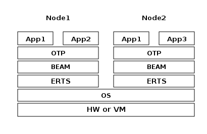
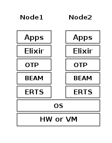
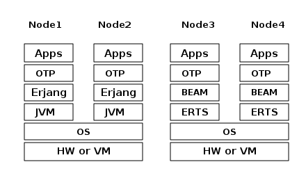
Your application(s) will run in one or more nodes, and the performance of your program will depend not only on your application code but also on all the layers below your code in the ERTS stack. In Figure 1 you can see the ERTS Stack illustrated with two Erlang nodes running on one machine.
If you are using Elixir there is yet another layer to the stack.
Let’s look at each layer of the stack and see how you can tune them to your application’s need.
At the bottom of the stack there is the hardware you are running on. The easiest way to improve the performance of your app is probably to run it on better hardware. You might need to start exploring higher levels of the stack if economical or physical constraints or environmental concerns won’t let you upgrade your hardware.
The two most important choices for your hardware is whether it is multicore and whether it is 32-bit or 64-bit. You need different builds of ERTS depending on whether you want to use multicore or not and whether you want to use 32-bit or 64-bit.
The second layer in the stack is the OS level. ERTS runs on most versions of Windows and most POSIX "compliant" operating systems, including Linux, FreeBSD, Solaris, and Mac OS X. Today most of the development of ERTS is done on Linux and OS X, and you can expect the best performance on these platforms. However, Ericsson has been using Solaris internally in many projects and ERTS has been tuned for Solaris for many years. Depending on your use case you might actually get the best performance on a Solaris system. The OS choice is usually not based on performance requirements, but is restricted by other factors. If you are building an embedded application you might be restricted to Raspbian and if you for some reason are building an end user or client application you might have to use Windows. The Windows port of ERTS has so far not had the highest priority and might not be the best choice from a performance or maintenance perspective. If you want to use a 64-bit ERTS you of course need to have both a 64-bit machine and a 64-bit OS. We will not cover many OS specific questions in this book, and most examples will be assuming that you run on Linux.
The third layer in the stack is the Erlang Runtime System. In our case this will be ERTS. This and the fourth layer, the Erlang Virtual Machine (BEAM), is what this book is all about.
The fifth layer, OTP, supplies the Erlang standard libraries. OTP
originally stood for "Open Telecom Platform" and was a number of
Erlang libraries supplying building blocks (such as supervisor,
gen_server and gen_tcp) for building robust applications (such as
telephony exchanges). Early on, the libraries and the meaning of OTP
got intermingled with all the other standard libraries shipped with
ERTS. Nowadays most people use OTP together with Erlang in
"Erlang/OTP" as the name for ERTS and all Erlang libraries shipped by
Ericsson. Knowing these standard libraries and how and when to use
them can greatly improve the performance of your application. This
book will not go into any details of the standard libraries and
OTP, there are many other books that cover these aspects.
If you are running an Elixir program the sixth layer provides the Elixir environment and the Elixir libraries.
Finally, the seventh layer (Apps) is your applications, and any third party libraries you use. The applications can use all the functionality provided by the underlying layers. Apart from upgrading your hardware this is probably the place where you most easily can improve your application’s performance. In Chapter 21 there are some hints and some tools that can help you profile and optimize your application. In Chapter 18 we will look at how to find the cause of crashing applications and how to find bugs in your application.
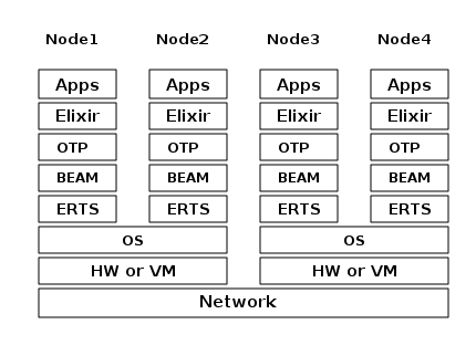
1.3.3. Distribution
One of the key insights by the Erlang language designers was that in order to build a system that works 24/7 you need to be able to handle hardware failure. Therefore you need to distribute your system over at least two physical machines. You do this by starting a node on each machine and then you can connect the nodes to each other so that processes can communicate with each other across the nodes just as if they were running in the same node. See Chapter 14 for details about distribution.
1.3.4. The Erlang Compiler
The Erlang Compiler is responsible for compiling Erlang source code,
from .erl files into BEAM virtual machine code.
The compiler is itself an Erlang application, written in Erlang and
compiled by itself into BEAM code. In a shipped Erlang-based system
(a release), the compiler might or might not be included depending
on whether that system needs to be able to compile code as well as run it.
To bootstrap the runtime system, the source distribution of Erlang includes
a number of precompiled BEAM files, including the compiler, in the
bootstrap and erts/preloaded directories.
For more information about the compiler see Chapter 2.
1.3.5. The Erlang Virtual Machine: BEAM
BEAM is the virtual machine used for executing Erlang code, just like the JVM is used for executing Java code. BEAM code runs in the context of an Erlang Node.
Just as ERTS is an implementation of a more general concept of a Erlang Runtime System so is BEAM an implementation of a more general Erlang Virtual Machine (EVM). There is no definition of what constitutes an EVM but BEAM actually has two levels of instructions: Generic Instructions and Specific Instructions. The generic instruction set could be seen as a blueprint for an EVM.
A detailed description of the BEAM can be found in Chapter 5 and the following chapters.
1.3.6. Processes
An Erlang process basically works like an OS process. Each process has its own private memory (a mailbox, a heap and a stack) and a process control block (PCB) with information about the process. Erlang processes are not like threads — they have no shared memory to modify, they can only communicate via messages, and from one process' point of view there is very little difference if another process runs in the same VM or is running on another node connected over the network. Erlang programs do not need locking or protected sections.
All Erlang code execution is done within the context of a process. One Erlang node can have many processes, which communicate through message passing and signals. Erlang processes can also communicate with processes on other Erlang nodes as long as the nodes are connected.
To learn more about processes and the PCB see Chapter 3.
1.3.7. Scheduling
The Scheduler is responsible for choosing the Erlang process to execute. Basically the scheduler keeps two queues, a ready queue of processes ready to run, and a waiting queue of processes waiting to receive a message.
The scheduler picks the first process from the ready queue and hands it to BEAM for execution of one time slice. BEAM preempts the running process when the time slice is used up and moves the process back to the end of the ready queue. If the process is blocked in a receive before the time slice is used up, it gets moved to the waiting queue instead. When a process in the waiting queue receives a message or gets a time out, it is moved to the ready queue.
Erlang is concurrent by nature, that is, each process is conceptually running at the same time as all other processes, but in reality the scheduler is just running one process at a time. Hence, even on a single core machine, and even if the underlying OS does not have preemption, the BEAM is still capable of running the same Erlang programs with hundreds of thousands of concurrent processes.
On a multicore machine, Erlang will automatically run more than one scheduler, in separate OS threads — usually one per physical core, each having their own run queues. If one scheduler runs out of work, it can take over some of the ready processes from the other schedulers. This way Erlang achieves true parallelism, without the programmer having to worry about it.
In reality the picture is more complicated with priorities among processes and the waiting queue is implemented through a timing wheel. All this and more is described in detail in Chapter 10.
1.3.8. The Erlang Tag Scheme
Erlang is a dynamically typed language, and the runtime system needs a way to keep track of the type of each data object. This is done with a tagging scheme. Each data object or pointer to a data object also has a tag with information about the data type of the object.
Basically, some bits of a pointer are reserved for the tag, and the VM can then determine the type of the object by looking at the bit pattern of the tag.
These tags are used for pattern matching and for type tests and for primitive operations, as well as by the garbage collector.
The complete tagging scheme is described in Chapter 4.
1.3.9. Memory Handling
Erlang uses automatic memory management and the programmer does not have to think about memory allocation and deallocation. Each process has a heap and a stack, and these can both grow and shrink as needed. There are no stack size limits to worry about, and no preallocated address ranges for stacks, as there can be for OS threads. Initially, both the stack and the heap for a process are quite small, which allows you to have many thousands or even millions of processes.
When a process runs out of heap space, the VM will first try to reclaim free heap space through garbage collection. The garbage collector will then go through the process stack and heap and copy live data to a new heap while throwing away all the data that is dead. If there still isn’t enough heap space, a new larger heap will be allocated and the live data is moved there.
The details of the current generational copying garbage collector, including the handling of reference counted binaries can be found in Chapter 11.
1.3.10. The Command Line Interface and the Interpreter
When you start an Erlang node with erl you get a command prompt.
This is the Erlang read eval print loop (REPL) or the command line
interface (CLI) or simply the Erlang shell.
You can type in Erlang expressions and execute them directly from the shell. In this case the code is not compiled to BEAM code and executed by the BEAM. Instead, the code is parsed and interpreted by the Erlang interpreter. In general, the interpreted code behaves exactly as compiled code, but there are a few subtle differences — in particular, the interpreted code is slower. These differences and all other aspects of the shell are explained in Chapter 17.
1.4. Alternative Erlang Implementations
This book is mainly concerned with the "standard" Erlang implementation by Ericsson/OTP called ERTS, but there are a few other implementations available and in this section we will look at some of them briefly.
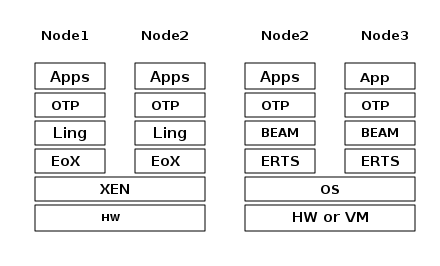
1.4.1. Erlang on Xen
Erlang on Xen (https://github.com/cloudozer/ling) is an Erlang implementation running directly on server hardware with no OS layer in between, only a thin Xen client.
Ling, the virtual machine of Erlang on Xen is almost 100% binary compatible with BEAM. In Figure 4 you can see how the Erlang on Xen implementation of the Erlang Solution Stack differs from the ERTS Stack. The thing to note here is that there is no operating system in the Erlang on Xen stack.
Since Ling implements the generic instruction set of BEAM, it can reuse the BEAM compiler from the OTP layer to compile Erlang to Ling.
1.4.2. Erjang
Erjang (https://github.com/trifork/erjang) is an Erlang implementation which runs
on the JVM. It loads .beam files and recompiles the code to Java .class
files. Erjang is almost 100% binary compatible with (generic) BEAM.
In Figure 5 you can see how the Erjang implementation of the Erlang Solution Stack differs from the ERTS Stack. The thing to note here is that JVM has replaced BEAM as the virtual machine and that Erjang provides the services of ERTS by implementing them in Java on top of the JVM.
Now that you have a basic understanding of all the major pieces of ERTS, and the necessary vocabulary, you can dive into the details of each component. If you are eager to understand a certain component, you can jump directly to that chapter. Or if you are really eager to find a solution to a specific problem, you could jump to the right chapter in Part II and try the different methods to tune, tweak, or debug your system.
2. The Compiler
This book will not cover the programming language Erlang, but since
the goal of the ERTS is to run Erlang code you will need to know how
to compile Erlang code. In this chapter we will cover the compiler
options needed to generate human readable BEAM code and how to add debug
information to the generated .beam file. At the end of the chapter
there is also a section on the Elixir compiler.
For those readers interested in compiling their own favorite language to ERTS this chapter will also contain detailed information about the different intermediate formats in the compiler and how to plug your compiler into the beam compiler backend. I will also present parse transforms and give examples of how to use them to tweak the Erlang language.
2.1. Compiling Erlang
Erlang is compiled from source code modules in .erl files
to binary .beam files.
The compiler can be run from the OS shell with the erlc command:
> erlc foo.erlThere are several options such as -o <Directory> for controlling the
general behaviour of erlc, mostly similar to C compiler options; see
https://www.erlang.org/doc/apps/erts/erlc_cmd.html for a complete
list. More specific compiler options begin with a plus sign, as in
+debug_info. These are Erlang terms passed straight to the compiler
application, and they may need quoting in the shell if they contain special
characters such as { or ". A full list of these options can be found in
the documentation of the compile module: see
http://www.erlang.org/doc/man/compile.html.
The compiler can also be invoked from the Erlang shell, either with the
shell shortcut command c(), which also loads the module afterwards , or
by calling compile:file(), which compiles but does not load. You can
specify the file name as an atom or a string, and you don’t need to include
the .erl extension:
1> c(foo).
{ok, foo}
or
1> compile:file(foo).
{ok, foo}
Both of these can take a list of options as a second argument. These are
the same terms that may be passed as +-options from erlc:
1> c(foo, [nowarn_unused_function, debug_info]).Normally the compiler will compile Erlang source code from a .erl
file and write the resulting binary beam code to a .beam file. You
can also get the resulting binary back as an Erlang term
by giving the option binary to compile:file() (but not to the c() shortcut):
1> compile:file(foo, [binary]).
{ok, foo, <<70,79,82,...>>}
Some options tell the compiler to stop after a certain stage of the compilation and produce the intermediate representation as output. For instance, to see what the program looks like after transformation to Core Erlang:
1> c(foo, [to_core]).
** Warning: No object file created - nothing loaded **
ok
The warning here is from the c() shell shortcut. Since no .beam object
file was created, there was no new version of the module to load. Instead,
you should now have a text file foo.core.
If we want to look at the result of preprocessing, we can pass the 'P'
option instead:
1> c(foo, ['P']).
** Warning: No object file created - nothing loaded **
ok
The output file foo.P now shows you what the Erlang source code looks
like after all include files have been read, macros have been substituted,
and conditional compilation directives like -ifdef have been evaluated.
In fact, the option binary
has been overloaded to mean “at the stage where the compiler stops,
return the intermediate format as a term instead of writing it to a file”.
If you for example want the compiler to return Core Erlang code you can
give the options [to_core, binary]:
1> compile:file(foo, [to_core,binary]).
{ok, foo, {c_module, ...}}
Note that you get the actual internal representation as Erlang terms in this case, not a chunk of text. Most internal representations have a corresponding prettyprinting function; for example:
1> {ok, foo, Core} = compile:file(foo, [to_core,binary]).
{ok, foo, {c_module, ...}}
2> io:put_chars(core_pp:format(Core)).
module 'foo' [...]
  ...
It is also possible to tell the compiler to pick up the compilation from a
later stage, for example from a .core source file, either using erlc:
> erlc foo.coreor directly from Erlang:
1> c(foo, [from_core]).
{ok, foo}
If you have some intermediate code as Erlang terms, you can pass it back straight to the compiler and tell it to continue working on it, like this:
1> {ok, foo, Core} = compile:file(foo, [to_core,binary]).
{ok, foo, {c_module, ...}}
3> {ok, foo, Bin} = compile:forms(Core, [from_core,binary]).
{ok,foo, <<70,79,82,...>>}
And finally, if you have a Beam module in binary form, you can load it directly into memory so you can run it:
4> code:load_binary(foo, "nopath", Bin).
{module,foo}
5> foo:f()
hello
6> code:which(foo).
"nopath"
(In this case you must tell the loader the module name as well as the string that the code server will report as the object file path, even if the binary was never stored in any file.)
This way it is possible to hook into the compiler at different points and
study the output, or modify it and pass it back, or even pass in low level
code that you have generated in some other way without having a
corresponding .erl file — and you can do all this without writing
anything to a file unless you want to.
2.2. Compiler Overview
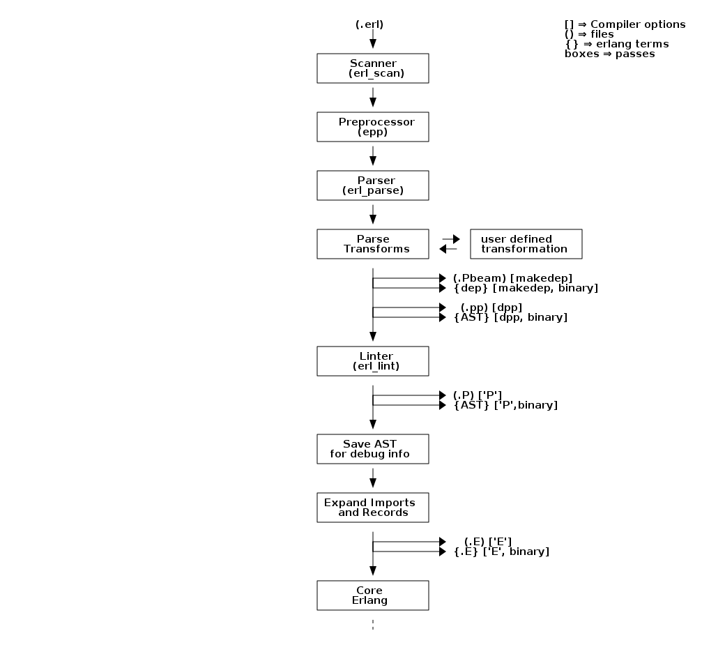
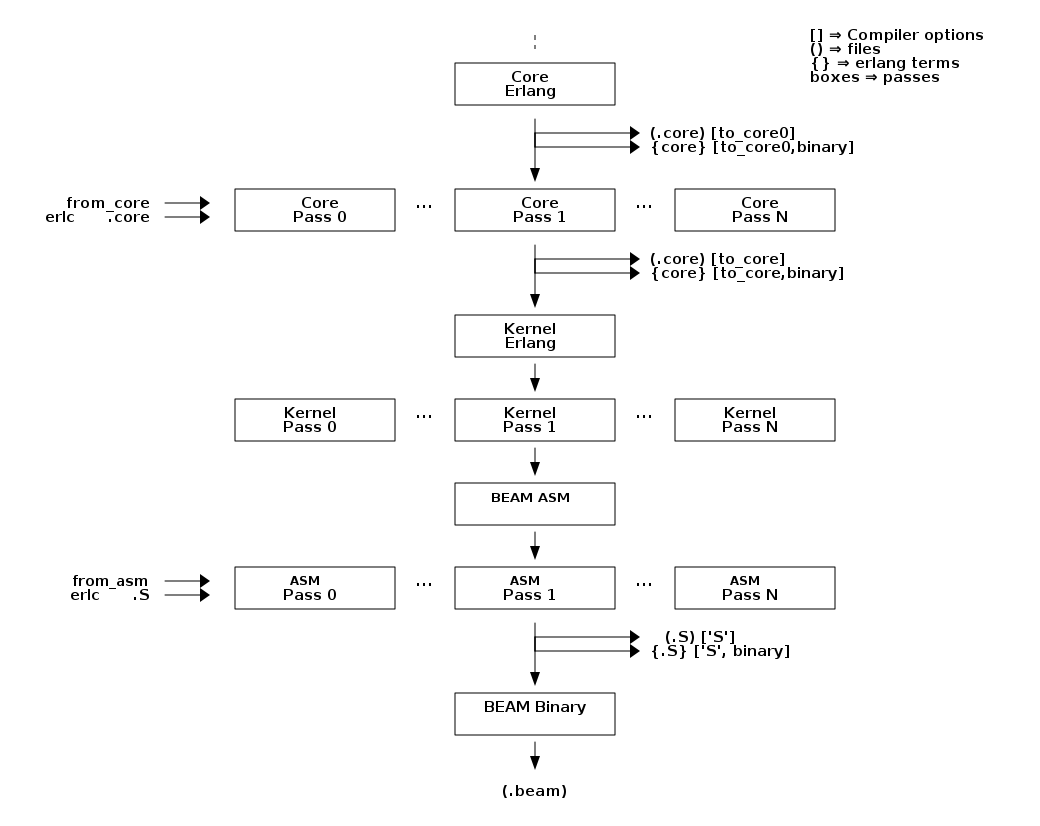
The compiler is made up of a number of passes. For readability, we divide these into two parts: the front end that takes Erlang source code and transforms it down to Core Erlang code (Figure 6), and the back end that continues from the Core Erlang level and transforms and optimizes the code down to BEAM bytecode (Figure 7).
If you want to see a complete and up to date list of compiler passes
you can run the function compile:options() in an Erlang shell.
The definitive source for information about the compiler is of course
the Erlang/OTP source code:
compile.erl
2.3. Generating Intermediate Output
Looking at the code produced by the compiler is a great help in trying to understand how the virtual machine works. Fortunately, the compiler can show us the intermediate code after each compiler pass and the final beam code.
Let us try out our newfound knowledge to look at the generated code.
 1> compile:options().
 dpp - Generate .pp file
 'P' - Generate .P source listing file
...
'E' - Generate .E source listing file
...
'S' - Generate .S file
Let us try with a small example program "world.erl":
-module(world).
-export([hello/0]).

-include("world.hrl").

hello() -> ?GREETING.
And the include file "world.hrl"
-define(GREETING, "hello world").If you now compile this with the 'P' option to get the parsed file you get a file "world.P":
2> c(world, ['P']).
** Warning: No object file created - nothing loaded **
ok
In the resulting .P file you can see a pretty printed version of
the code after the preprocessor (and parse transformation) has been
applied:
-file("world.erl", 1).

-module(world).

-export([hello/0]).

-file("world.hrl", 1).

-file("world.erl", 4).

hello() ->
    "hello world".
To see how the code looks after all source code transformations are
done, you can compile the code with the 'E'-flag.
3> c(world, ['E']).
** Warning: No object file created - nothing loaded **
ok
This gives us an .E file, in this case all compiler directives have
been removed, any records have been expanded to tuples, any uses of function imports
have been expanded to explicit remote calls,
and the built in functions module_info/{1,2} have been
added to the source:
-vsn("\002").

-file("world.erl", 1).

-file("world.hrl", 1).

-file("world.erl", 5).

hello() ->
    "hello world".

module_info() ->
    erlang:get_module_info(world).

module_info(X) ->
    erlang:get_module_info(world, X).
We will make use of the 'P' and 'E' options when we look at parse transforms later in Section 2.5.
Before we get into all the other intermediate stages, we will take a look
at the final generated BEAM code, in its human readable “assembler” form.
By giving the option 'S' to the compiler you get a .S file with Erlang
terms for each BEAM instruction in the code.
3> c(world, ['S']).
** Warning: No object file created - nothing loaded **
ok
The file world.S should look something like this:
{module, world}.  %% version = 0

{exports, [{hello,0},{module_info,0},{module_info,1}]}.

{attributes, []}.

{labels, 7}.


{function, hello, 0, 2}.
  {label,1}.
    {line,[{location,"world.erl",6}]}.
    {func_info,{atom,world},{atom,hello},0}.
  {label,2}.
    {move,{literal,"hello world"},{x,0}}.
    return.


{function, module_info, 0, 4}.
  {label,3}.
    {line,[]}.
    {func_info,{atom,world},{atom,module_info},0}.
  {label,4}.
    {move,{atom,world},{x,0}}.
    {line,[]}.
    {call_ext_only,1,{extfunc,erlang,get_module_info,1}}.


{function, module_info, 1, 6}.
  {label,5}.
    {line,[]}.
    {func_info,{atom,world},{atom,module_info},1}.
  {label,6}.
    {move,{x,0},{x,1}}.
    {move,{atom,world},{x,0}}.
    {line,[]}.
    {call_ext_only,2,{extfunc,erlang,get_module_info,2}}.
Since this is a file with dot (.) separated Erlang terms, you can
easily read the file back into the Erlang shell with:
{ok, BEAM_Code} = file:consult("world.S").
As you can see, the assembler code mostly follows the layout of the original source code.
The first instruction defines the module name of the code. The version
mentioned in the comment (%% version = 0) is the version of the
opcode format (as given by beam_opcodes:format_number/0).
Then comes a list of exports and any compiler attributes (none in this example) much like in any Erlang source module.
The first real beam-like instruction is {labels, 7} which tells the
VM the number of labels in the code to make it possible to allocate
room for all labels in one pass over the code.
After that there is the actual code for each function. The first instruction gives us the function name, the arity, and the entry point as a label number. You’ll notice that the entry point is not the first label in the function — before it there are some instructions that define metadata for the function. These are not executed at runtime.
You can use the 'S' option with great effect to help you understand
how the BEAM works, and we will use it like that in later chapters. It
is also invaluable if you develop your own language that you compile
to the BEAM through Core Erlang, to see the generated code.
2.4. Compiler Passes
In the following sections we will go through most of the compiler passes shown in Figure 6 and Figure 7. For a language designer targeting the BEAM this is interesting since it will show you what you can accomplish with the different approaches: macros, parse transforms, Core Erlang, and BEAM code, and how they depend on each other.
When tuning Erlang code, it is good to know what optimizations are applied when, and how you can look at generated code before and after optimizations.
2.4.1. Compiler Pass: The Erlang Preprocessor (epp)
The compilation starts with tokenization (or scanning) and
preprocessing. The preprocessor epp reads a file and calls the tokenizer
erl_scan to expand the text into a sequence of separate tokens
rather than characters, discarding whitespace and comments. It then
processes macro definitions and conditional compilation directives, and
substitutes uses of macros.
When the preprocessor finds an include statement, it reads and tokenizes the
named include file, inserts the resulting token sequence instead of the
include statement, and then processes that as well so that files can
include each other recursively. When it switches between one file and
another, the preprocessor inserts -file annotations, as we saw in the
example above, so that later passes can know where a particular piece of
code came from:
...
-file("world.hrl", 1).

-file("world.erl", 4).
...
Note that when an include file like world.hrl gets processed, there may
be no actual code inserted, since include files often contain only macro
definitions and preprocessor conditionals. All that is left are the
annotations saying “we are now at line 1 of the header file” and “we are
now back at line 4 in the original source file”.
Note that all this means that epp works on the token level (just
like the C/C++ preprocessor cpp), so it
is not a pure string replacement processor (as for example m4).
You cannot use Erlang macros to define your own arbitrary syntax; a macro
will expand as a separate token from its surrounding characters, so
you can’t concatenate a macro and a character to a token:
-define(plus,+).
t(A,B) -> A?plus+B.
This will expand to
t(A,B) -> A + + B.and not
t(A,B) -> A ++ B.On the other hand since macro expansion is done on the token stream before the actual parsing, you do not need to have a valid Erlang term in the right hand side of the macro, as long as you use it in a way that gives you a valid term in the end. E.g.:
-define(p,o, o]).
 t() -> [f,?p.
which will expand to the token sequence
t ( ) -> [ f , o , o ] .There are few real usages for this other than to win the obfuscated Erlang code contest. The main point to remember is that you can’t really use the Erlang preprocessor to define a language with a syntax that differs from Erlang.
2.4.2. Compiler Pass: The Erlang Parser
The parser erl_parse gets the final token sequence from the
preprocessor and checks it against the Erlang grammar, producing an
abstract syntax tree or AST (see
http://www.erlang.org/doc/apps/erts/absform.html ) representing the
program as a data structure instead of as a sequential text.
2.4.3. Compiler Pass: Parse Transformations
A parse transform is a function that works on the AST. After the compiler has done the initial tokenization, preprocessing and parsing, and assuming there were no errors so far, it will call the parse transform function if one has been declared, passing it the current AST and expecting to get a modified AST back.
This means that you can’t change the Erlang syntax fundamentally, because the input must still be accepted by the Erlang parser, but you can change the semantics by modifying the code as you like.
A parse transform is declared like this, in the module where it is to be used:
-compile({parse_transform, my_pt}).The compiler will then try to call my_pt:parse_transform(Forms, Options)
as an extra pass. It is possible to use multiple parse transforms in the
same module; they will simply be executed in order.
Parse transforms are used by libraries such as Mnesia (for its QLC syntax), EUnit, Merl, and others. In Section 2.5 we will demonstrate a full example of how you can implement your own parse transform.
2.4.4. Compiler Pass: Linter
The term “linter” originally meant a tool that was an add-on to a compiler — like a lint filter in a clothes dryer — checking for stylistic errors and antipatterns and other things that the compiler itself did not check (because in those days compilers had very little memory available and were focused on speed). As computers got faster, however, the linter got moved into the compiler itself as a pass that you wanted to run all the time, not just occasionally.
In the Erlang compiler, the linter erl_lint is the stage that
does most of the checking of the source code, after parsing and transforms
are done. (This means that parse transforms may only return an AST that the
linter will accept.)
The linter checks for errors, such as undefined variables and functions, as well as generating warnings for correct but suspicious code, such as "export_all flag enabled".
2.4.5. Compiler Pass: Save AST
In order to enable debugging of a module you must “debug compile” the
module, that is pass the option debug_info to the compiler. The
abstract syntax tree will then be saved by the “Save AST” pass, until the
end of the compilation where it will be included in the .beam file for
purposes of setting breakpoints, single stepping etc. The code is then
running interpreted, not compiled.
It is important to note that the code is saved before any optimisations are applied, so if there is a bug in an optimisation pass in the compiler and you run interpreted code in the debugger you will get a different behavior. If you are implementing your own compiler optimisations, this can trip you up badly.
2.4.6. Compiler Pass: Expand
In the expand phase, source level Erlang constructs such as records are
expanded to lower level erlang constructs. This strips compiler directives,
replaces record syntax with operations on tuples, expands uses of function
imports to explicit remote calls, and adds the built in functions
module_info/{1,2} to the code.
2.4.7. Compiler Pass: Core Erlang
Core Erlang is a strict functional language suitable for compiler optimizations. It makes code transformations easier by reducing the number of ways to express the same operation. One way it does this is by introducing let and letrec expressions to make scoping more explicit. The compiler does several passes on the core level.
Core Erlang can be a good target for a language you want to run in ERTS. It changes very seldom and it contains all aspects of Erlang in a clean way. If you target the BEAM instruction set directly, you will have to deal with many more details, and that instruction set usually changes slightly between each major release of ERTS. If you on the other hand target Erlang directly you will be more restricted in what you can describe, and you may also have to deal with more details, since Core Erlang is a cleaner language.
Note however that targeting plain Erlang gives you more compile time checking that your generated code is well behaved. By generating Core Erlang directly, you may manage to find corner cases that the Erlang compiler never has encountered before; there is a greater responsibility on you to generate correct code.
To compile an Erlang file to core you can give the option to_core.
This outputs the resulting Core Erlang program to a file with
the extension .core. To compile a Core Erlang program from a .core
file you can give the option from_core to the compiler.
1> c(world, to_core).
** Warning: No object file created - nothing loaded **
ok
2> c(world, from_core).
{ok,world}
Note that the .core files are text files written in the human
readable core format. To get the core program as an Erlang term
you can add the binary option to the compilation.
2.4.8. Compiler Pass: Kernel Erlang
Kernel Erlang is a flat version of Core Erlang with a few differences. For example, each variable is unique and the scope is a whole function. Pattern matching is compiled to more primitive operations. The kernel representation does not have a well defined file format and you should not expect it to be stable.
2.4.9. Compiler Pass: BEAM Assembly Code
The last stage of a normal compilation is the external BEAM assembly code format, as a sequence of individual BEAM instructions represented as Erlang terms. Some low level optimizations such as dead code elimination and peep hole optimisations are done on this level.
The BEAM code is described in detail in Chapter 7 and Appendix B
2.4.10. Compiler Pass: BEAM Binary Format
The BEAM assembly code is finally packed into the binary transport format
which can be written to a .beam file, sent over the network, or loaded
directly into memory through code:load_binary/3. See
Chapter 6] for details.
2.5. Writing a Parse Transform
The easiest way to tweak the Erlang language is through Parse Transformations (or parse transforms). Parse Transformations come with all sorts of warnings, like this note in the OTP documentation:
| Programmers are strongly advised not to engage in parse transformations and no support is offered for problems encountered. |
When you use a parse transform you are basically writing an extra pass in the compiler and that can if you are not careful lead to very unexpected results. But to use a parse transform you have to declare the usage in the module using it, and it will be local to that module, so as far as compiler tweaks goes this one is relatively safe.
The biggest problem with parse transforms as I see it is that you are inventing your own syntax, and it will make it more difficult for anyone else reading your code. At least until your parse transform has become as popular and widely used as e.g. QLC.
OK, so you know now that you shouldn’t use it, but if you have to anyway, let’s give you an example of how to do it.
Lets say for example that you for some reason would like to write json code directly in your Erlang code, then you are in luck since the tokens of json and of Erlang are basically the same. Also, since the Erlang compiler does most of its sanity checks in the linter pass which follows the parse transform pass, you can allow an AST which does not represent valid Erlang.
To write a parse transform you need to write an Erlang module (lets
call it p) which exports the function parse_transform/2. This
function is called by the compiler during the parse transform pass if
the module being compiled (lets call it m) contains the compiler
option {parse_transform, p}. The arguments to the function is the
AST of the module m and the compiler options given to the call to the
compiler.
|
Note that you will not get any compiler options given in the file, which is a bit of a nuisance since you can’t give options to the parse transform from the code. The compiler does not expand compiler options until the expand pass which occurs after the parse transform pass. |
The documentation of the abstract format is somewhat dense and it is
quite hard to get a grip on the abstract format by reading the
documentation. I encourage you to use the syntax_tools and
especially erl_syntax_lib for any serious work on the AST.
Here we will develop a simple parse transform just to get an
understanding of the AST. Therefore we will work directly on the AST
and use the old reliable io:format approach instead of syntax_tools.
First we create an example of what we would like to be able to compile json_test.erl:
-module(json_test).
-compile({parse_transform, json_parser}).
-export([test/1]).

test(V) ->
    <<{{
      "name"  : "Jack (\"Bee\") Nimble",
      "format": {
                 "type"      : "rect",
                 "widths"     : [1920,1600],
                 "height"    : (-1080),
                 "interlace" : false,
                 "frame rate": V
                }
      }}>>.
Then we create a minimal parse transform module json_parser.erl:
-module(json_parser).
-export([parse_transform/2]).

parse_transform(AST, _Options) ->
  io:format("~p~n", [AST]),
  AST.
This identity parse transform returns an unchanged AST but it also prints it out so that you can see what an AST looks like.
> c(json_parser).
{ok,json_parser}
2> c(json_test).
[{attribute,1,file,{"./json_test.erl",1}},
 {attribute,1,module,json_test},
 {attribute,3,export,[{test,1}]},
 {function,5,test,1,
  [{clause,5,
    [{var,5,'V'}],
    [],
    [{bin,6,
      [{bin_element,6,
        {tuple,6,
         [{tuple,6,
           [{remote,7,{string,7,"name"},{string,7,"Jack (\"Bee\") Nimble"}},
            {remote,8,
             {string,8,"format"},
             {tuple,8,
              [{remote,9,{string,9,"type"},{string,9,"rect"}},
               {remote,10,
                {string,10,"widths"},
                {cons,10,
                 {integer,10,1920},
                 {cons,10,{integer,10,1600},{nil,10}}}},
               {remote,11,{string,11,"height"},{op,11,'-',{integer,11,1080}}},
               {remote,12,{string,12,"interlace"},{atom,12,false}},
               {remote,13,{string,13,"frame rate"},{var,13,'V'}}]}}]}]},
        default,default}]}]}]},
 {eof,16}]
./json_test.erl:7: illegal expression
./json_test.erl:8: illegal expression
./json_test.erl:5: Warning: variable 'V' is unused
error
The compilation of json_test fails since the module contains invalid
Erlang syntax, but you get to see what the AST looks like. Now we can
just write some functions to traverse the AST and rewrite the json
code into Erlang code.[1]
-module(json_parser).
-export([parse_transform/2]).

parse_transform(AST, _Options) ->
    json(AST, []).

-define(FUNCTION(Clauses), {function, Label, Name, Arity, Clauses}).

%% We are only interested in code inside functions.
json([?FUNCTION(Clauses) | Elements], Res) ->
    json(Elements, [?FUNCTION(json_clauses(Clauses)) | Res]);
json([Other|Elements], Res) -> json(Elements, [Other | Res]);
json([], Res) -> lists:reverse(Res).

%% We are interested in the code in the body of a function.
json_clauses([{clause, CLine, A1, A2, Code} | Clauses]) ->
    [{clause, CLine, A1, A2, json_code(Code)} | json_clauses(Clauses)];
json_clauses([]) -> [].


-define(JSON(Json), {bin, _, [{bin_element
                                         , _
                                         , {tuple, _, [Json]}
                                         , _
                                         , _}]}).

%% We look for: <<"json">> = Json-Term
json_code([])                     -> [];
json_code([?JSON(Json)|MoreCode]) -> [parse_json(Json) | json_code(MoreCode)];
json_code(Code)                   -> Code.

%% Json Object -> [{}] | [{Label, Term}]
parse_json({tuple,Line,[]})            -> {cons, Line, {tuple, Line, []}};
parse_json({tuple,Line,Fields})        -> parse_json_fields(Fields,Line);
%% Json Array -> List
parse_json({cons, Line, Head, Tail})   -> {cons, Line, parse_json(Head),
                                                       parse_json(Tail)};
parse_json({nil, Line})                -> {nil, Line};
%% Json String -> <<String>>
parse_json({string, Line, String})     -> str_to_bin(String, Line);
%% Json Integer -> Integer
parse_json({integer, Line, Integer})   -> {integer, Line, Integer};
%% Json Float -> Float
parse_json({float, Line, Float})       -> {float, Line, Float};
%% Json Constant -> true | false | null
parse_json({atom, Line, true})         -> {atom, Line, true};
parse_json({atom, Line, false})        -> {atom, Line, false};
parse_json({atom, Line, null})         -> {atom, Line, null};

%% Variables, should contain Erlang encoded Json
parse_json({var, Line, Var})         -> {var, Line, Var};
%% Json Negative Integer or Float
parse_json({op, Line, '-', {Type, _, N}}) when Type =:= integer
                                             ; Type =:= float ->
                                          {Type, Line, -N}.
%% parse_json(Code)                  -> io:format("Code: ~p~n",[Code]), Code.

-define(FIELD(Label, Code), {remote, L, {string, _, Label}, Code}).

parse_json_fields([], L) -> {nil, L};
%% Label : Json-Term  --> [{<<Label>>, Term} | Rest]
parse_json_fields([?FIELD(Label, Code) | Rest], _) ->
    cons(tuple(str_to_bin(Label, L), parse_json(Code), L)
         , parse_json_fields(Rest, L)
         , L).


tuple(E1, E2, Line)    -> {tuple, Line, [E1, E2]}.
cons(Head, Tail, Line) -> {cons, Line, Head, Tail}.

str_to_bin(String, Line) ->
    {bin
     , Line
     , [{bin_element
         , Line
         , {string, Line, String}
         , default
         , default
        }
       ]
    }.
And now we can compile json_test without errors:
1> c(json_parser).
{ok,json_parser}
2> c(json_test).
{ok,json_test}
3> json_test:test(42).
[{<<"name">>,<<"Jack (\"Bee\") Nimble">>},
{<<"format">>,
  [{<<"type">>,<<"rect">>},
   {<<"widths">>,[1920,1600]},
   {<<"height">>,-1080},
   {<<"interlace">>,false},
   {<<"frame rate">>,42}]}]
The AST generated by parse_transform/2 must correspond to valid
Erlang code unless you apply several parse transforms, which is
possible. The validity of the code is checked by the following
compiler pass.
2.6. Other Compiler Tools
There are a number of tools available to help you work with code generation and code manipulation. These tools are written in Erlang and not really part of the runtime system but they are very nice to know about if you are implementing another language on top of the BEAM.
In this section we will cover three of the most useful code tools: the lexer — Leex, the parser generator — Yecc, and a general set of functions to manipulate abstract forms — Syntax Tools.
2.6.1. Leex
Leex is the Erlang lexer generator.
The lexer generator takes a description of a DFA from a definitions
file xrl and produces an Erlang
program that matches tokens described by the DFA.
The details of how to write a DFA definition for a tokenizer
is beyond the scope of this book. For a thorough explanation
I recommend the "Dragon book" ([DragonBook]).
Other good resources are the man and info entry for flex, the lexer program
that inspired leex, and the leex documentation itself.
If you have info and flex installed you can read the full manual by typing:
> info flex
The online Erlang documentation also has the leex manual (see yecc.html).
We can use the lexer generator to create an Erlang program which recognizes JSON tokens. By looking at the JSON definition http://www.ecma-international.org/publications/files/ECMA-ST/ECMA-404.pdf we can see that there are only a handful of tokens that we need to handle.
Definitions.

Digit         = [0-9]
Digit1to9     = [1-9]
HexDigit      = [0-9a-f]
UnescapedChar = [^\"\\]
EscapedChar   = (\\\\)|(\\\")|(\\b)|(\\f)|(\\n)|(\\r)|(\\t)|(\\/)
Unicode       = (\\u{HexDigit}{HexDigit}{HexDigit}{HexDigit})
Quote         = [\"]
Delim         = [\[\]:,{}]
Space         = [\n\s\t\r]

Rules.

{Quote}{Quote} : {token, {string, TokenLine, ""}}.
{Quote}({EscapedChar}|({UnescapedChar})|({Unicode}))+{Quote} :
  {token, {string, TokenLine, drop_quotes(TokenChars)}}.

null  : {token, {null,  TokenLine}}.
true  : {token, {true,  TokenLine}}.
false : {token, {false, TokenLine}}.

{Delim} : {token, {list_to_atom(TokenChars), TokenLine}}.

{Space} : skip_token.

-?{Digit1to9}+{Digit}*\.{Digit}+((E|e)(\+|\-)?{Digit}+)? :
  {token, {number, TokenLine, list_to_float(TokenChars)}}.
-?{Digit1to9}+{Digit}* :
  {token, {number, TokenLine, list_to_integer(TokenChars)+0.0}}.

Erlang code.
-export([t/0]).

drop_quotes([$" | QuotedString]) -> literal(lists:droplast(QuotedString)).
literal([$\\,$" | Rest]) ->
  [$"|literal(Rest)];
literal([$\\,$\\ | Rest]) ->
  [$\\|literal(Rest)];
literal([$\\,$/ | Rest]) ->
  [$/|literal(Rest)];
literal([$\\,$b | Rest]) ->
  [$\b|literal(Rest)];
literal([$\\,$f | Rest]) ->
  [$\f|literal(Rest)];
literal([$\\,$n | Rest]) ->
  [$\n|literal(Rest)];
literal([$\\,$r | Rest]) ->
  [$\r|literal(Rest)];
literal([$\\,$t | Rest]) ->
  [$\t|literal(Rest)];
literal([$\\,$u,D0,D1,D2,D3|Rest]) ->
  Char = list_to_integer([D0,D1,D2,D3],16),
  [Char|literal(Rest)];
literal([C|Rest]) ->
  [C|literal(Rest)];
literal([]) ->[].

t() ->
  {ok,
   [{'{',1},
    {string,2,"no"},
    {':',2},
    {number,2,1.0},
    {'}',3}
   ],
   4}.
By using the Leex compiler we can compile this DFA to Erlang code,
and by giving the option dfa_graph we also produce a dot-file
which can be viewed with e.g. Graphviz.
1> leex:file(json_tokens, [dfa_graph]).
{ok, "./json_tokens.erl"}
2>
You can view the DFA graph (Figure 8) using for example dotty:
> dotty json_tokens.dot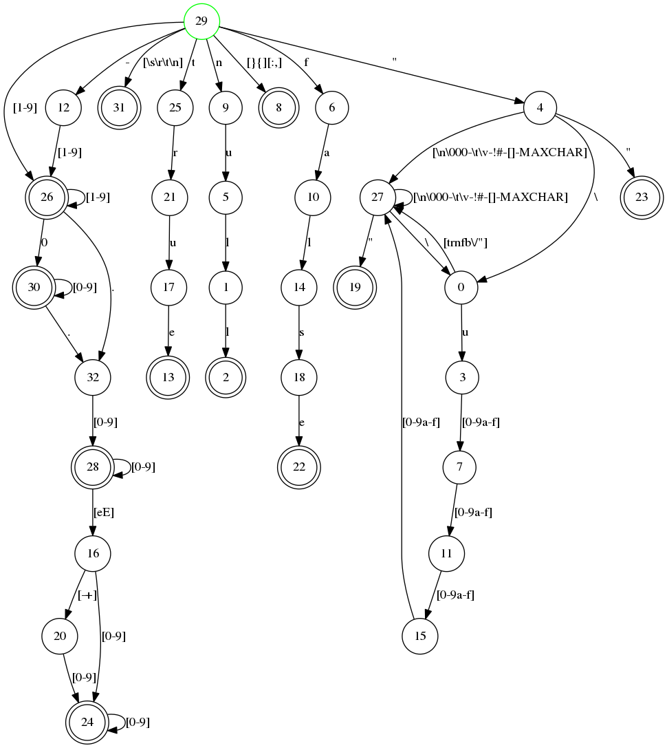
We can try our tokenizer on an example json file (test.json).
{
    "no" : 1,
    "name"  : "Jack \"Bee\" Nimble",
    "escapes" : "\b\n\r\t\f\//\\",
    "format": {
        "type"      : "rect",
        "widths"    : [1920,1600],
        "height"    : -1080,
        "interlace" : false,
        "unicode"   : "\u002f",
        "frame rate": 4.5
    }
}
First we need to compile our tokenizer, then we read the file
and convert it to a string. Finally we can use
the string/1 function that leex generates to tokenize the test file.
2> c(json_tokens).
{ok,json_tokens}.
3> f(File), f(L), {ok, File} = file:read_file("test.json"), L = binary_to_list(File), ok.
ok
4> f(Tokens), {ok, Tokens,_} = json_tokens:string(L), hd(Tokens).
{'{',1}
5>
The shell function f/1 tells the shell to forget a variable
binding. This is useful if you want to try a command that binds a
variable multiple times, for example as you are writing the lexer and
want to try it out after each rewrite. We will look at the shell
commands in detail in the later chapter.
Armed with a tokenizer for JSON we can now write a json parser using the parser generator Yecc.
2.6.2. Yecc
Yecc is a parser generator for Erlang. The name comes from Yacc (Yet Another Compiler Compiler) the canonical parser generator for C. The modern open source equivalent is Bison, which is often used with Flex.
Now that we have a lexer for JSON terms we can write a parser using
yecc.
Nonterminals value values object array pair pairs.

Terminals number string true false null '[' ']' '{' '}' ',' ':'.

Rootsymbol value.

value -> object  :  '$1'.
value -> array   :  '$1'.
value -> number  :  get_val('$1').
value -> string  :  get_val('$1').
value -> 'true'  :  get_val('$1').
value -> 'null'  :  get_val('$1').
value -> 'false' :  get_val('$1').

object -> '{' '}' : #{}.
object -> '{' pairs '}' : '$2'.

pairs -> pair : '$1'.
pairs -> pair ',' pairs : maps:merge('$1', '$3').

pair -> string ':' value : #{ get_val('$1') => '$3' }.

array -> '[' ']' : {}.
array -> '[' values ']' : list_to_tuple('$2').

values -> value : [ '$1' ].
values -> value ',' values : [ '$1' | '$3' ].


Erlang code.

get_val({_,_,Val}) -> Val;
get_val({Val, _}) -> Val.
Then we can use yecc to generate an Erlang program that implements
the parser, and call the parse/1 function provided with the tokens
generated by the tokenizer as an argument.
5> yecc:file(yecc_json_parser), c(yecc_json_parser).
{ok,yexx_json_parser}
6> f(Json), {ok, Json} = yecc_json_parser:parse(Tokens).
{ok,#{"escapes" => "\b\n\r\t\f////",
      "format" => #{"frame rate" => 4.5,
        "height" => -1080.0,
        "interlace" => false,
        "type" => "rect",
        "unicode" => "/",
        "widths" => {1920.0,1.6e3}},
       "name" => "Jack \"Bee\" Nimble",
       "no" => 1.0}}
The tools Leex and Yecc are nice when you want to compile your own complete language to the Erlang virtual machine. By combining them with Syntax tools and specifically Merl you can manipulate the Erlang Abstract Syntax tree, either to generate Erlang code or to change the behaviour of Erlang code.
2.7. Syntax Tools and Merl
Syntax Tools is a set of libraries for manipulating the internal representation of Erlang’s Abstract Syntax Trees (ASTs).
The syntax tools applications also includes the metaprogramming utility Merl . With Merl you can very easily manipulate the syntax tree and write parse transforms in Erlang code.
You can find the documentation for Syntax Tools on the Erlang.org site: http://erlang.org/doc/apps/syntax_tools/chapter.html.
2.8. Compiling Elixir
Another approach to writing your own language on top of the BEAM is to use the macro programming facilities in Elixir. Elixir compiles to BEAM code through the Erlang abstract syntax tree.
With Elixir’s defmacro you can define your own Domain Specific Language, directly in Elixir.
3. Processes
The concept of lightweight processes is the essence of Erlang and the BEAM; they are what makes BEAM stand out from other virtual machines. In order to understand how the BEAM (and Erlang and Elixir) works you need to know the details of how processes work, which will help you understand the central concept of the BEAM, including what is easy and cheap for a process and what is hard and expensive.
Almost everything in the BEAM is connected to the concept of processes and in this chapter we will learn more about these connections. We will expand on what we learned in the introduction and take a deeper look at concepts such as memory management, message passing, and in particular scheduling.
An Erlang process is very similar to an OS process. It has its own address space, it can communicate with other processes through signals and messages, and the execution is controlled by a preemptive scheduler.
When you have a performance problem in an Erlang or Elixir system the problem is very often stemming from a problem within a particular process or from an imbalance between processes. There are of course other common problems such as bad algorithms or memory problems which we will look at in other chapters. Still, being able to pinpoint the process which is causing the problem is always important, therefore we will look at the tools available in the Erlang Runtime System for process inspection.
We will introduce the tools throughout the chapter as we go through how a process and the scheduler works, and then we will bring all tools together for an exercise at the end.
3.1. What is a Process?
A process is an isolated entity where code execution occurs. A process protects your system from errors in your code by isolating the effect of the error to the process executing the faulty code.
The runtime comes with a number of tools for inspecting processes to help us find bottlenecks, problems and overuse of resources. These tools will help you identify and inspect problematic processes.
3.1.1. Listing Processes from the Shell
Let us dive right in and look at which processes we have
in a running system. The easiest way to do that is to
just start an Erlang shell and issue the shell command i().
In Elixir you can call the function in the shell_default module as
:shell_default.i.
$ erl
Erlang/OTP 19 [erts-8.1] [source] [64-bit] [smp:4:4] [async-threads:10]
               [kernel-poll:false]

Eshell V8.1  (abort with ^G)
1> i().
Pid                   Initial Call                     Heap     Reds Msgs
Registered            Current Function                 Stack
<0.0.0>               otp_ring0:start/2                 376      579    0
init                  init:loop/1                         2
<0.1.0>               erts_code_purger:start/0          233        4    0
erts_code_purger      erts_code_purger:loop/0             3
<0.4.0>               erlang:apply/2                    987   100084    0
erl_prim_loader       erl_prim_loader:loop/3              5
<0.30.0>              gen_event:init_it/6               610      226    0
error_logger          gen_event:fetch_msg/5               8
<0.31.0>              erlang:apply/2                   1598      416    0
application_controlle gen_server:loop/6                   7
<0.33.0>              application_master:init/4         233       64    0
                      application_master:main_loop/2      6
<0.34.0>              application_master:start_it/4     233       59    0
                      application_master:loop_it/4        5
<0.35.0>              supervisor:kernel/1               610     1767    0
kernel_sup            gen_server:loop/6                   9
<0.36.0>              erlang:apply/2                   6772    73914    0
code_server           code_server:loop/1                  3
<0.38.0>              rpc:init/1                        233       21    0
rex                   gen_server:loop/6                   9
<0.39.0>              global:init/1                     233       44    0
global_name_server    gen_server:loop/6                   9
<0.40.0>              erlang:apply/2                    233       21    0
                      global:loop_the_locker/1            5
<0.41.0>              erlang:apply/2                    233        3    0
                      global:loop_the_registrar/0         2
<0.42.0>              inet_db:init/1                    233      209    0
inet_db               gen_server:loop/6                   9
<0.44.0>              global_group:init/1               233       55    0
global_group          gen_server:loop/6                   9
<0.45.0>              file_server:init/1                233       79    0
file_server_2         gen_server:loop/6                   9
<0.46.0>              supervisor_bridge:standard_error/ 233       34    0
standard_error_sup    gen_server:loop/6                   9
<0.47.0>              erlang:apply/2                    233       10    0
standard_error        standard_error:server_loop/1        2
<0.48.0>              supervisor_bridge:user_sup/1      233       54    0
                      gen_server:loop/6                   9
<0.49.0>              user_drv:server/2                 987     1975    0
user_drv              user_drv:server_loop/6              9
<0.50.0>              group:server/3                    233       40    0
user                  group:server_loop/3                 4
<0.51.0>              group:server/3                    987    12508    0
                      group:server_loop/3                 4
<0.52.0>              erlang:apply/2                   4185     9537    0
                      shell:shell_rep/4                  17
<0.53.0>              kernel_config:init/1              233      255    0
                      gen_server:loop/6                   9
<0.54.0>              supervisor:kernel/1               233       56    0
kernel_safe_sup       gen_server:loop/6                   9
<0.58.0>              erlang:apply/2                   2586    18849    0
                      c:pinfo/1                          50
Total                                                 23426   220863    0
                                                        222
ok
The i/0 function prints out a list of all processes in the system.
Each process gets two lines of information. The first two lines
of the printout are the headers telling you what the information
means. As you can see you get the Process ID (Pid) and the name of the
process if any, as well as information about the code where the process
was started and where it is currently executing. You also get information about the
heap and stack size and the number of reductions and messages in
the process. In the rest of this chapter we will learn in detail
what a stack, a heap, a reduction and a message are. For now we
can just assume that if there is a large number for the heap size,
then the process uses a lot of memory and if there is a large number
for the reductions then the process has executed a lot of code.
We can further examine a process with the i/3 function. Let
us take a look at the code_server process. We can see in the
previous list that the process identifier (pid) of the code_server
is <0.36.0>. By calling i/3 with the three numbers of
the pid we get this information:
2> i(0,36,0).
[{registered_name,code_server},
 {current_function,{code_server,loop,1}},
 {initial_call,{erlang,apply,2}},
 {status,waiting},
 {message_queue_len,0},
 {messages,[]},
 {links,[<0.35.0>]},
 {dictionary,[]},
 {trap_exit,true},
 {error_handler,error_handler},
 {priority,normal},
 {group_leader,<0.33.0>},
 {total_heap_size,46422},
 {heap_size,46422},
 {stack_size,3},
 {reductions,93418},
 {garbage_collection,[{max_heap_size,#{error_logger => true,
                                       kill => true,
                                       size => 0}},
                      {min_bin_vheap_size,46422},
                      {min_heap_size,233},
                      {fullsweep_after,65535},
                      {minor_gcs,0}]},
 {suspending,[]}]
3>
We got a lot of information from this call and in the rest of this
chapter we will learn in detail what most of these items mean. The
first line tells us that the process has been given a name
code_server. Next we can see in which function the process is
currently executing or suspended (current_function)
and the name of the function in which the process started executing
(initial_call).
We can also see that the process is suspended waiting for messages
({status,waiting}) and that there are no messages in the
mailbox ({message_queue_len,0}, {messages,[]}). We will look
closer at how message passing works later in this chapter.
The fields priority, suspending, reductions, links,
trap_exit, error_handler, and group_leader control the process
execution, error handling, and IO. We will look into this a bit more
when we introduce the Observer.
The last few fields (dictionary, total_heap_size, heap_size,
stack_size, and garbage_collection) give us information about the
process memory usage. We will look at the process memory areas in
detail in chapter Chapter 11.
Another, even more intrusive way of getting information
about processes is to use the process information given
by the BREAK menu: Ctrl+c p [enter]. Note that while
you are in the BREAK state the whole node freezes.
3.1.2. Programmatic Process Probing
The shell functions just print the information about the
process but you can actually get this information as data,
so you can write your own tools for inspecting processes.
You can get a list of all processes with erlang:processes/0,
and information about a specific process with
erlang:process_info/1. We can also use the function
whereis/1 to get a pid from a name:
1> Ps = erlang:processes().
[<0.0.0>,<0.1.0>,<0.4.0>,<0.30.0>,<0.31.0>,<0.33.0>,
 <0.34.0>,<0.35.0>,<0.36.0>,<0.38.0>,<0.39.0>,<0.40.0>,
 <0.41.0>,<0.42.0>,<0.44.0>,<0.45.0>,<0.46.0>,<0.47.0>,
 <0.48.0>,<0.49.0>,<0.50.0>,<0.51.0>,<0.52.0>,<0.53.0>,
 <0.54.0>,<0.60.0>]
2> CodeServerPid = whereis(code_server).
<0.36.0>
3> erlang:process_info(CodeServerPid).
[{registered_name,code_server},
 {current_function,{code_server,loop,1}},
 {initial_call,{erlang,apply,2}},
 {status,waiting},
 {message_queue_len,0},
 {messages,[]},
 {links,[<0.35.0>]},
 {dictionary,[]},
 {trap_exit,true},
 {error_handler,error_handler},
 {priority,normal},
 {group_leader,<0.33.0>},
 {total_heap_size,24503},
 {heap_size,6772},
 {stack_size,3},
 {reductions,74260},
 {garbage_collection,[{max_heap_size,#{error_logger => true,
                                       kill => true,
                                       size => 0}},
                      {min_bin_vheap_size,46422},
                      {min_heap_size,233},
                      {fullsweep_after,65535},
                      {minor_gcs,33}]},
 {suspending,[]}]
By getting process information as data we can write code
to analyze or sort the data as we please. If we grab all
processes in the system (with erlang:processes/0) and
then get information about the heap size of each process
(with erlang:process_info(P, total_heap_size)) we can
then construct a list with pid and heap size and sort
it on heap size:
1> lists:reverse(lists:keysort(2,[{P,element(2,
    erlang:process_info(P,total_heap_size))}
    || P <- erlang:processes()])).
[{<0.36.0>,24503},
 {<0.52.0>,21916},
 {<0.4.0>,12556},
 {<0.58.0>,4184},
 {<0.51.0>,4184},
 {<0.31.0>,3196},
 {<0.49.0>,2586},
 {<0.35.0>,1597},
 {<0.30.0>,986},
 {<0.0.0>,752},
 {<0.33.0>,609},
 {<0.54.0>,233},
 {<0.53.0>,233},
 {<0.50.0>,233},
 {<0.48.0>,233},
 {<0.47.0>,233},
 {<0.46.0>,233},
 {<0.45.0>,233},
 {<0.44.0>,233},
 {<0.42.0>,233},
 {<0.41.0>,233},
 {<0.40.0>,233},
 {<0.39.0>,233},
 {<0.38.0>,233},
 {<0.34.0>,233},
 {<0.1.0>,233}]
2>
You might notice that many processes have a heap size of 233 words, that is because it is the default starting heap size of a process.
See the documentation of the module erlang for a full description of
the information available from process_info/2:
https://erlang.org/doc/apps/erts/erlang.html#process_info/2
Notice how the process_info/1 function only returns a subset of all
the information available for the process and how the process_info/2
function can be used to fetch extra information. As an example, to
extract the backtrace for the code_server process above, we could
run:
3> process_info(whereis(code_server), backtrace).
{backtrace,<<"Program counter: 0x00000000161de900 (code_server:loop/1 + 152)\nCP: 0x0000000000000000 (invalid)\narity = 0\n\n0"...>>}
See the three dots at the end of the binary above? That means that the
output has been truncated. A useful trick to see the whole value is to
wrap the above function call using the rp/1 function:
4> rp(process_info(whereis(code_server), backtrace)).An alternative is to use the io:put_chars/1 function, as follows:
5> {backtrace, Backtrace} = process_info(whereis(code_server), backtrace).
{backtrace,<<"Program counter: 0x00000000161de900 (code_server:loop/1 + 152)\nCP: 0x0000000000000000 (invalid)\narity = 0\n\n0"...>>}
6> io:put_chars(Backtrace).
Due to its verbosity, the output for commands 4> and 6> has not
been included here, but feel free to try the above commands in your
Erlang shell.
3.1.3. Using Observer to Inspect Processes
A third way of examining processes is with the Observer. Observer is an extensive graphical interface for inspecting the Erlang Runtime System. We will use the Observer throughout this book to examine different aspects of the system.
To start Observer, Erlang needs to have been compiled with WxWidgets
support, and the observer and wx applications must be available on the
node. You probably do not want that on your production system, but Observer
is made with this in mind. You can start Observer from an Erlang that has
been built with support for it, and then go into the “Nodes” menu and
select “Connect node” and you will be able to Observe the connected node
instead of the local node.
|
For now, we will just start Observer from the Erlang shell like this:
7> observer:start().or from the Elixir shell with :observer.start. For debugging a live
system, you probably want to launch a temporary Erlang node just for
running Observer, using the -hidden flag to prevent the inspected nodes
from seeing the observer node:
$ erl -hidden -sname observer -run observerWhen Observer is started it will show you a system overview, see the following screen shot:
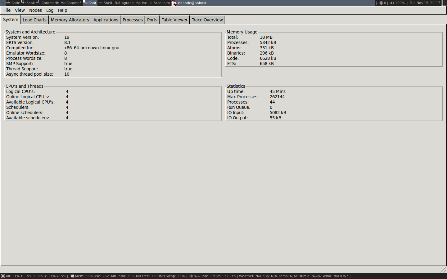
We will go over some of this information in detail later in
this and the next chapter. For now we will just use Observer to look
at the running processes. First we take a look at the
Applications tab which shows the supervision tree of the running system:
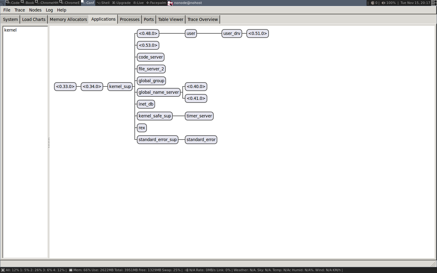
Here we get a graphical view of how the processes are linked. This is a very nice way to get an overview of how a system is structured. You also get a nice feeling of processes as isolated entities floating in space connected to each other through links.
To actually get some useful information about the processes
we switch to the Processes tab:
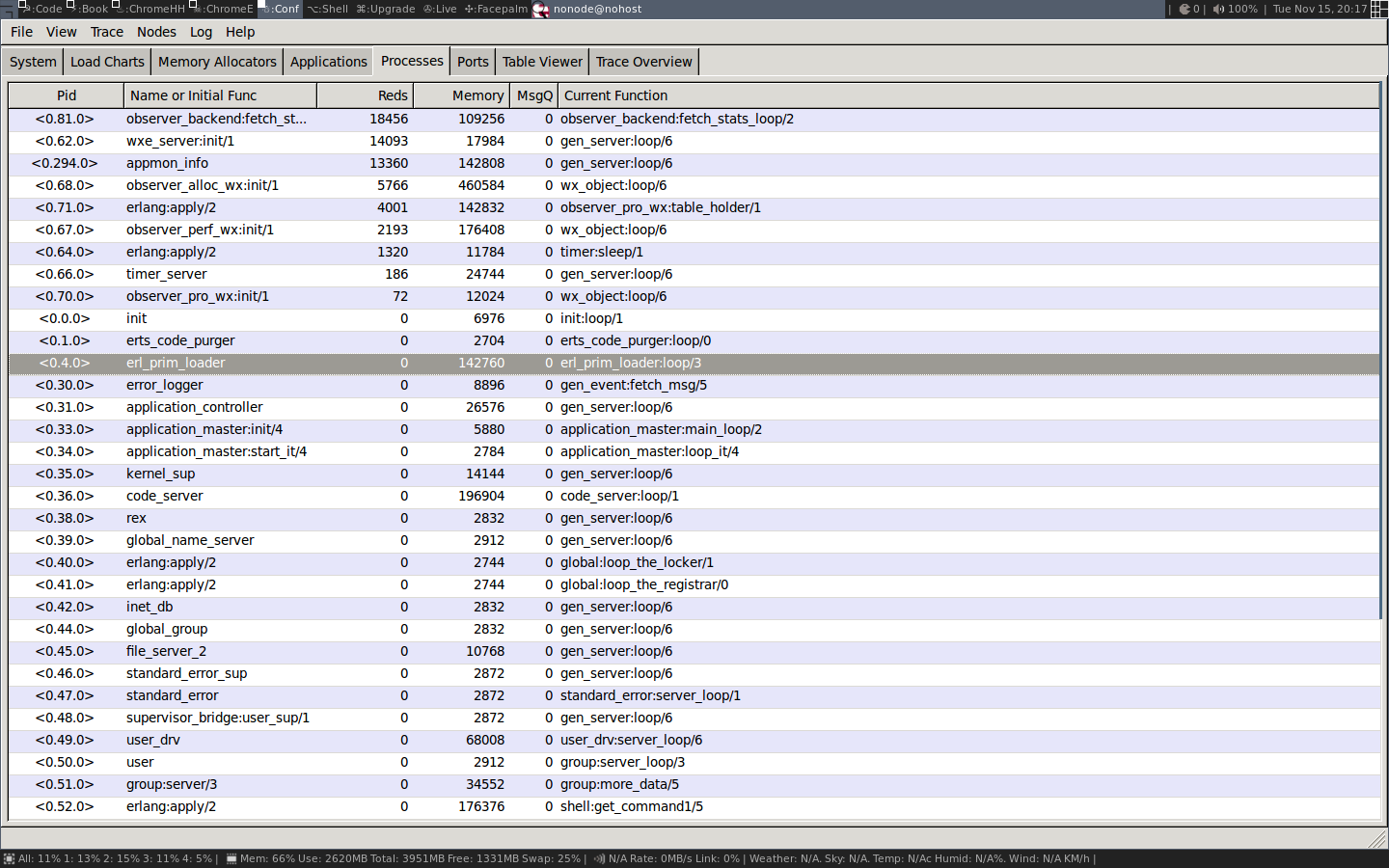
In this view we get basically the same information as with
i/0 in the shell. We see the pid, the registered name,
number of reductions, memory usage and number of messages
and the current function.
We can also look into a process by double clicking on its
row, for example on the code server, to get the kind of
information you can get with process_info/2:
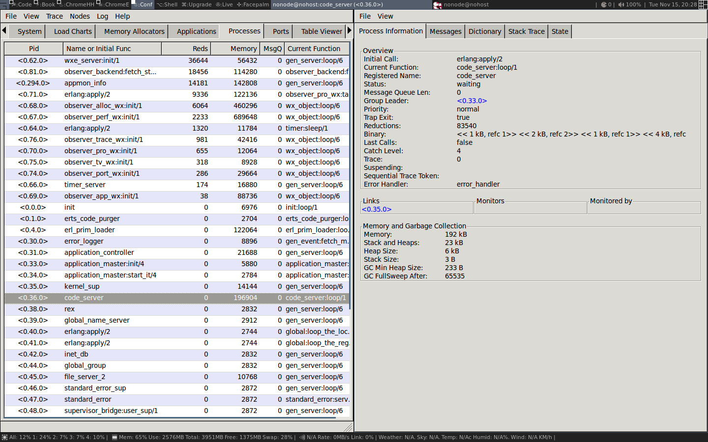
We will not go through what all this information means right now, but if you keep on reading all will eventually be revealed.
Now that we have a basic understanding of what a process is and some tools to find and inspect processes in a system, we are ready to dive deeper to learn how a process is implemented.
3.2. Processes Are Just Memory
A process is basically four blocks of memory: a stack, a heap, a message area, and the Process Control Block (the PCB).
The stack is used for keeping track of program execution by storing return addresses, for passing arguments to functions, and for keeping local variables. Larger structures, such as lists and tuples are stored on the heap.
The message area, also called the mailbox, is used to store messages sent to the process from other processes. The process control block is used to keep track of the state of the process.
See Figure 9 for an illustration of a process as memory.
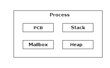
This picture of a process is very much simplified, and we will go through a number of iterations of more refined versions to get to a more accurate picture.
The stack, the heap, and the mailbox are all dynamically allocated and can grow and shrink as needed. We will see exactly how this works in later chapters. The PCB on the other hand is statically allocated and contains a number of fields that controls the process.
We can inspect some of these memory regions with built-in introspection calls.
For example, erlang:process_info/2 lets you ask a process for its stack_size,
heap_size, total_heap_size, or a raw backtrace binary,
while the current_stacktrace item returns the stack as a structured
list of {M,F,A,Location} tuples that you can pattern-match or pretty-print yourself.
The shell helper c:bt(Pid) is just a convenience wrapper around erlang:process_display(Pid, backtrace).
Combined with process_info items such as memory or reductions,
these queries give a view of a process’s stack, heap, and PCB-like fields.
For a deeper, byte-level view the runtime ships with the Emulator Toolbox for Pathologists (ETP)—a collection of GDB macros (etp-stackdump, etp-heapdump, etp-process-info, and friends) that walk live BEAM data structures in a paused VM or core dump.
See Appendix A for more information on how to build the a debug version of the Erlang runtime system with ETP support.
We can see the context of the stack of a process with erlang:process_display/2:
1> erlang:process_display(self(), backtrace).
Program counter: 0x00007fdf9baa2e78 (erlang:self/0 + 32)

0x00007fdedf247480 Return addr 0x00007fdf9baa2118 (erlang:process_display/2 + 128)
y(0)     []
y(1)     backtrace
y(2)     <0.89.0>

0x00007fdedf2474a0 Return addr 0x00007fdf9bbb7644 (erl_eval:do_apply/7 + 308)
y(0)     none
y(1)     []

0x00007fdedf2474b8 Return addr 0x00007fdf9bf0e430 (shell:exprs/7 + 536)
y(0)     []
y(1)     []
y(2)     []
y(3)     []
y(4)     cmd
y(5)     []
y(6)     {value,#Fun<shell.5.46532814>}
y(7)     {eval,#Fun<shell.23.46532814>}
y(8)     #Ref<0.908573933.3456499713.143140>
y(9)     []

0x00007fdedf247510 Return addr 0x00007fdf9bf0dc60 (shell:eval_exprs/7 + 152)
y(0)     []
y(1)     []
y(2)     []
y(3)     []
y(4)     <0.88.0>
y(5)     Catch 0x00007fdf9bf0dd0e (shell:eval_exprs/7 + 326)

0x00007fdedf247548 Return addr 0x00007fdf9bf0d87c (shell:eval_loop/4 + 564)
y(0)     #Ref<0.908573933.3456499713.143140>
y(1)     #Ref<0.908573933.3456499713.143160>
y(2)     <0.88.0>

0x00007fdedf247568 Return addr 0x00007fdf9ba2d1f8 (<terminate process normally>)
true
We will look closer at the values on the stack and the heap in Chapter 4.
You can inspect the heap of a process with RTP and a debug version of the BEAM.
Assuming you have built a debug version:
$ERL_TOP/bin/cerl -debug -rgdb
GNU gdb (Ubuntu 15.0.50.20240403-0ubuntu1) 15.0.50.20240403-git
...
Reading symbols from beam.debug.smp...
%---------------------------------------------------------------------------
% Use etp-help for a command overview and general help.
%
% To use the Erlang support module, the environment variable ROOTDIR
% must be set to the toplevel installation directory of Erlang/OTP,
% so the etp-commands file becomes:
%     $ROOTDIR/erts/etc/unix/etp-commands
% Also, erl and erlc must be in the path.
%---------------------------------------------------------------------------
etp-set-max-depth 20
etp-set-max-string-length 100
--------------- System Information ---------------
OTP release: 24
ERTS version: 12.3.2.17
Arch: x86_64-pc-linux-gnu
Endianness: Little
Word size: 64-bit
BeamAsm support: yes
--Type <RET> for more, q to quit, c to continue without paging--
SMP support: yes
Thread support: yes
Kernel poll: Supported
Debug compiled: yes
Lock checking: yes
Lock counting: no
System not initialized
--------------------------------------------------
Then you can start the BEAM with run.
(gdb) run
Starting program: /home/happi/hh/theBeamBook/otp24/bin/x86_64-pc-linux-gnu/beam.debug.smp -- -root /home/happi/hh/theBeamBook/otp24 -progname /home/happi/hh/theBeamBook/otp24/bin/cerl -debug -- -home /home/happi -- -emu_type debug

This GDB supports auto-downloading debuginfo from the following URLs:
  <https://debuginfod.ubuntu.com>
Enable debuginfod for this session? (y or [n]) y
Debuginfod has been enabled.
To make this setting permanent, add 'set debuginfod enabled on' to .gdbinit.
warning: could not find '.gnu_debugaltlink' file for /lib/x86_64-linux-gnu/libtinfo.so.6
[Thread debugging using libthread_db enabled]
Using host libthread_db library "/lib/x86_64-linux-gnu/libthread_db.so.1".
[New Thread 0x7fffb6baf6c0 (LWP 2185)]
...
[New Thread 0x7fff9f4fa6c0 (LWP 2232)]
Erlang/OTP 24 [erts-12.3.2.17] [source] [64-bit] [smp:16:16] [ds:16:16:10] [async-threads:1] [jit] [type-assertions] [debug-compiled] [lock-checking]

Eshell V12.3.2.17  (abort with ^G)
1>
Let us start a process with some dynamic data on the heap:
-module(mini_proc).
-export([wait/0]).

wait() ->
  X = {timestamp, erlang:timestamp()},
  receive _ -> X end,
  X.
Now we can compile and start that process in the shell within the debugger:
1> c(mini_proc).
{ok,mini_proc}
9> P3 = spawn(mini_proc, wait, []).
<0.101.0>
By pressing Ctrl+c we get back to the debugger:
    Thread 1 "beam.debug.smp" received signal SIGINT, Interrupt.
                                                                [Switching to Thread 0x7ffff79b3c40 (LWP 2170)]
(gdb)
I had some problem with the ETP commands unless I was in a scheduler thread, so let’s switch to one and list the processes:
(gdb) thread 7
[Switching to thread 7 (Thread 0x7fffb40b96c0 (LWP 2191))]
(gdb) etp-processes
---
  Pix: 0
  Pid: <0.0.0>
  State: prq-prio-normal | usr-prio-normal | act-prio-normal

  Flags: trap-exit
  Registered name: init
  Current function: unknown
  I: #Cp<init:loop/1+0x64>
  Heap size: 987
  Old-heap size: 987
  Mbuf size: 38
  Msgq len: 0 (inner=0, outer=0)
  Msgq Flags: on-heap
  Parent: []
  Pointer: (Process*)0x5555561301c8

...

---
  Pix: 808
  Pid: <0.101.0>
  State: prq-prio-normal | usr-prio-normal | act-prio-normal

  Flags:
  Current function: unknown
  I: #Cp<0x7fffb53711dc>
  Heap size: 233
  Old-heap size: 0
  Mbuf size: 0
  Msgq len: 0 (inner=0, outer=0)
  Msgq Flags: on-heap
  Parent: <0.93.0>
  Pointer: (Process*)0x7fff9ed6e030
---
  Pix: 816
  Pid: <0.102.0>
  State: prq-prio-normal | usr-prio-normal | act-prio-normal

  Flags:
  Current function: unknown
  I: #Cp<io:execute_request/3+0x1a4>
  Heap size: 233
  Old-heap size: 0
  Mbuf size: 0
  Msgq len: 0 (inner=0, outer=0)
  Msgq Flags: on-heap
  Parent: <0.79.0>
  Pointer: (Process*)0x7fff9ed6dce8
---
(gdb)
We see the address of the '<0.101.0>' process in the Pointer field.
We can use the etp-stackdump and etp-heapdump commands to
inspect the stack and heap of the process. The etp-stackdump
command takes a process pointer as an argument.
(gdb) set $p = ((Process *) 0x7fff9ed6e030)
(gdb) etp-stackdump $p
% Stacktrace (3)
I: #Cp<0x7fffb53711dc>.
0: {timestamp,{1747,147859,212377}}.
1: #Cp<0x7fffb4c14a78>.
2: #Cp<0x7fffb4c14a78>.
(gdb) etp-heapdump $p
% heapdump (7):
 0x7fff9eaf8278: | H:   3-tuple | I:      1747 | I:    147859 | I:    212377 | H:   2-tuple |    timestamp | B:0x9eaf827a
(gdb)
As expected the stack and the heap contains a 2-tuple with the 3-tuple timestamp: {timestamp, {1747,147859,212377}}.
3.3. The PCB
The Process Control Block contains all the fields that control the behaviour and current state of a process. In this section and the rest of the chapter we will go through the most important fields. We will leave out some fields that have to do with execution and tracing from this chapter, instead we will cover those in Chapter 5.
We can see most of the fields in the PCB by just printing the value of what the process pointer points to:
print *((Process *) 0x7fff9ed6e030)
$2 = {common =
      {id = 3470333576787,
       refc = {atmc = {counter = 1}, sint = 1},
       tracer = 59, trace_flags = 167772160,
       timer = {counter = 0},
       u = {alive = {started_interval = 263, reg = 0x0, links = 0x0,
                    lt_monitors = 0x0, monitors = 0x0},
                   release = {later = 263, func = 0x0, data = 0x0, next = 0x0}}},
      htop = 0x7fff9eaf82b0,
      stop = 0x7fff9eaf89a8,
      fcalls = 3998,
      freason = 0,
      fvalue = 59,
      heap = 0x7fff9eaf8278,
      hend = 0x7fff9eaf89c0,
      abandoned_heap = 0x0,
      heap_sz = 233,
      min_heap_size = 233,
      min_vheap_size = 46422,
      max_heap_size = 3,
      arity = 0,
      arg_reg = 0x7fff9ed6e0f8,
      max_arg_reg = 6,
      def_arg_reg = {588235, 322955, 59, 14178673876263027908, 14178673876263027908, 4000},
      i = 0x7fffb53711dc <mini_proc:wait/0+140>,
      catches = 0, rcount = 0, schedule_count = 0,
      reds = 6, flags = 0, group_leader = 2267742733347, ftrace = 59, next = 0x555556142888,
      uniq = 0,
      sig_qs = {first = 0x0, last = 0x7fff9ed6e170, save = 0x7fff9ed6e170, cont = 0x0,
                cont_last = 0x7fff9ed6e188,
                nmsigs = {next = 0x0, last = 0x0},
                recv_mrk_blk = 0x0, len = 0, flags = 2},
      bif_timers = 0x0, dictionary = 0x0,
      seq_trace_clock = 0, seq_trace_lastcnt = 0, seq_trace_token = 59,
      u = {real_proc = 0x8f9cb, terminate = 0x8f9cb,
           initial = {module = 588235, function = 322955, arity = 0}},
      current = 0x0, parent = 3195455669715, static_flags = 0,
      high_water = 0x7fff9eaf8278,
      old_hend = 0x0,
      old_htop = 0x0,
      old_heap = 0x0,
      gen_gcs = 0,
      max_gen_gcs = 65535,
      off_heap = {first = 0x0, overhead = 0},
      mbuf = 0x0, live_hf_end = 0xfffffffffffffff8, msg_frag = 0x0, mbuf_sz = 0,
      psd = {counter = 0},
      bin_vheap_sz = 46422, bin_old_vheap_sz = 46422, bin_old_vheap = 0,
      sys_task_qs = 0x0, dirty_sys_tasks = 0x0,
      state = {counter = 42}, dirty_state = {counter = 0},
      sig_inq = {first = 0x0, last = 0x7fff9ed6e2a8, len = 0,
                 nmsigs = {next = 0x0, last = 0x0}},
      trace_msg_q = 0x0,lock = {flags = {counter = 0},
                                queue = {0x0, 0x0, 0x0, 0x0, 0x0},
                                locked = {{counter = 0}, {counter = 0}, {counter = 0},
                                          {counter = 0}, {counter = 0}}},
      scheduler_data = 0x0, run_queue = {counter = 140736249294720},
      last_htop = 0x7fff9eaf8298, last_mbuf = 0x0, heap_hfrag = 0x0, last_old_htop = 0x0,
      debug_reds_in = 4000
     }
If you want to dig even deeper than we will go in this chapter you can
look at the C source code. The PCB is implemented as a C struct called process in the file
erl_process.h for OTP19
or erl_process.h
for the latest version.
The field id contains the process ID (or PID).
'id = 3470333576787' which is '0b110010100000000000000000000000011001010011' in binary.
The process ID is an Erlang term and hence tagged (See Chapter 4). This means
that the 4 least significant bits are a tag (0011). In the
code section there is a module for inspecting Erlang terms
(see show.erl in the online appendix)
which we will cover in
the chapter on types. We can use it now to examine the
type of a tagged word though.
4> show:tag_to_type(3470333576787).
pid
5>
The fields htop and stop are pointers to the top of the heap and
the stack, that is, they are pointing to the next free slots on the heap
or stack. The fields heap (start) and hend points to the start and
the stop of the whole heap, and heap_sz gives the size of the heap
in words. That is hend - heap = heap_sz * 8 on a 64 bit machine and
hend - heap = heap_sz * 4 on a 32 bit machine.
The field min_heap_size is the size, in words, that the heap starts
with and which it will not shrink smaller than, the default value is
233.
We can now refine the picture of the process heap with the fields from the PCB that controls the shape of the heap, see Figure 10:
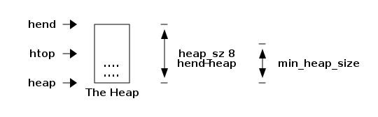
But wait, how come we have a heap start and a heap end, but no start and stop for the stack? That is because the BEAM uses a trick to save space and pointers by allocating the heap and the stack together. It is time for our first revision of our process as memory picture. The heap and the stack are actually just one memory area, as illustrated in Figure 11:
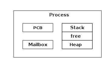
The stack grows towards lower memory addresses and the heap towards higher memory, so we can also refine the picture of the heap by adding the stack top pointer to the picture, see Figure 12:
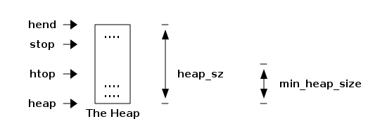
If the pointers htop and stop should meet, the
process has run out of free memory and will have to call the garbage
collector to free up memory.
3.4. The Garbage Collector (GC)
The heap memory management schema is to use a per process copying generational garbage collector. When there is no more space on the heap (or the stack, since they share the allocated memory block), the garbage collector kicks in to free up memory.
The GC allocates a new memory area called the to space. Then it goes through the stack to find all live roots and follows each root and copies the data on the heap to the new heap. Finally it also copies the stack to the new heap and frees up the old memory area.
The GC is controlled by these fields in the PCB:
    Eterm *high_water;
    Eterm *old_hend;     /* Heap pointers for generational GC. */
    Eterm *old_htop;
    Eterm *old_heap;
    Uint max_heap_size;  /* Maximum size of heap (in words). */
    Uint16 gen_gcs;      /* Number of (minor) generational GCs. */
    Uint16 max_gen_gcs;	 /* Max minor gen GCs before fullsweep. */
Since the garbage collector is generational it will use a heuristic to just look at
new data most of the time. That is, in what is called a minor collection, the GC
only looks at the top part of the stack and moves new data to the new
heap. Old data, i.e., data allocated below the high_water mark
on the heap (see Figure 13), is moved to a special
area called the old heap.
Most of the time, then, there is
another heap area for
each process: the old heap, handled by the fields old_heap,
old_htop and old_hend in the PCB. This almost brings us back to
our original picture of a process as four memory areas, as shown in
Figure 13:
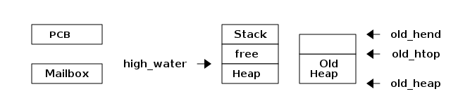
When a process starts there is no old heap, but as soon as young data has matured to old data and there is a garbage collection, the old heap is allocated. The old heap is garbage collected when there is a major collection, also called a full sweep. See Chapter 11 for more details of how garbage collection works. In that chapter we will also look at how to track down and fix memory related problems.
3.5. Mailboxes and Message Passing
Process communication is done through message passing. A process send is implemented so that a sending process copies the message from its own heap to the mailbox of the receiving process.
In the early days of Erlang, concurrency was implemented solely by Erlang’s own scheduler performing the task switching. We will talk more about concurrency in the section about the scheduler later in this chapter, for now it is worth noting that in the first version of Erlang there was no parallelism and there could only be one process running at the time. In that version the sending process could write data directly into the heap of the receiving process, without locking.
3.5.1. Sending Messages in Parallel
When multicore systems were introduced and the Erlang implementation
was extended with more than one scheduler running processes in parallel it
was no longer safe to write directly into another process' heap without
taking the main lock of the receiver. At this time the concept of
m-bufs was introduced (also called heap fragments). An m-buf is
a memory area
outside of a process heap where other processes can
safely write data. If a sending process can not get the lock, it would
write to the m-buf instead. When all data of a message has been
copied to the m-buf, the message is linked to the process through the
mailbox. The linking (LINK_MESSAGE in
erl_message.h)
appends the message to the receiver’s
message queue.
The garbage collector would then copy the messages onto the process' heap. To reduce the pressure on the GC the mailbox is divided into two lists, one containing seen messages and one containing new messages. The GC does not have to look at the new messages since we know they will survive (they are still in the mailbox) and that way we can avoid some copying.
3.6. Lock Free Message Passing
In Erlang 19 a new per process setting was introduced, message_queue_data,
which can take the values on_heap or off_heap. When set to on_heap
the sending process will first try to take the main lock of the
receiver and if it succeeds the message will be copied directly
onto the receiver’s heap. This can only be done if the receiver is
suspended and if no other process has grabbed the lock to send to
the same process. If the sender can not obtain the lock it will
allocate a heap fragment and copy the message there instead.
If the flag is set to off_heap the sender will not try to get the
lock and instead write directly to a heap fragment. This will reduce
lock contention but allocating a heap fragment is more expensive than
writing directly to the already allocated process heap and it can
lead to larger memory usage. There might be a large empty heap allocated
and still new messages are written to new fragments.
With on_heap allocation all the messages, both directly allocated on
the heap and messages in heap fragments, will be copied by the GC. If
the message queue is large and many messages are not handled and
therefore still are live, they will be promoted to the old heap and
the size of the process heap will increase, leading to higher
memory usage.
All messages are added to a linked list (the mailbox) when the
message has been copied to the receiving process. If the message
is copied to the heap of the receiving process the message is
linked in to the internal message queue (or seen messages)
and examined by the GC.
In the off_heap allocation scheme new messages are placed in
the “external” message in-queue and ignored by the GC.
3.6.1. Memory Areas for Messages
We can now revise our picture of the process as four memory areas
once more. Now the process is made up of five memory areas (two
mailboxes) and a varying number of heap fragments (m-bufs), as
shown in Figure 14:
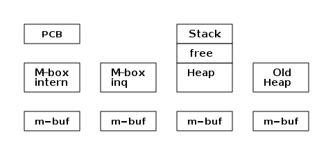
Each mailbox consists of a length and two pointers, stored in the fields
msg.len, msg.first, msg.last for the internal queue and msg_inq.len,
msg_inq.first, and msg_inq.last for the external in queue. There is
also a pointer to the next message to look at (msg.save) to implement
selective receive.
3.6.2. The Process of Sending a Message to a Process
We will ignore the distribution case for now, that is we will not
consider messages sent between Erlang nodes. Imagine two processes
P1 and P2. Process P1 wants to send a message (Msg) to process
P2, as illustrated by Figure 15:
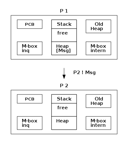
Process P1 will then take the following steps:
-
Calculate the size of
Msg. -
Allocate space for the message (on or off
P2's heap as described before). -
Copy
MsgfromP1's heap to the allocated space. -
Allocate and fill in an
ErlMessagestruct wrapping up the message. -
Link in the
ErlMessageeither in theErlMsgQueueor in theErlMsgInQueue.
If process P2 is suspended and no other process is trying to
send a message to P2 and there is space on the heap and the
allocation strategy is on_heap the message will directly end up
on the heap, as in Figure 16:
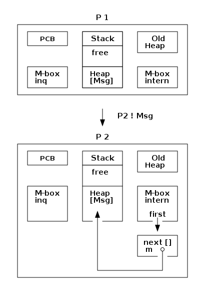
If P1 can not get the main lock of P2 or there is not enough space
on P2 's heap and the allocation strategy is on_heap the message
will end up in an m-buf but linked from the internal mailbox, as in
Figure 17:
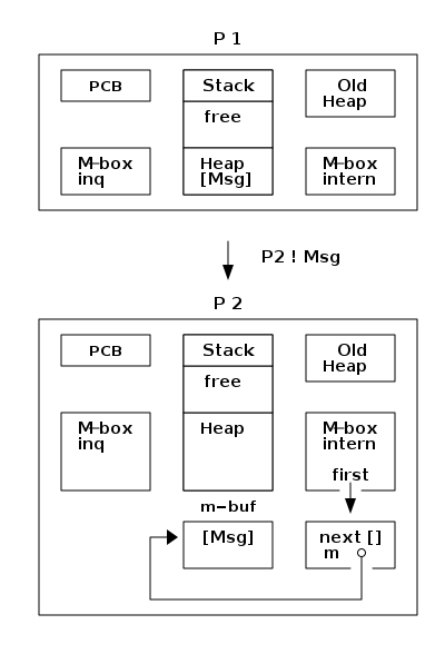
After a GC the message will be moved into the heap.
If the allocation strategy is off_heap the message
will end up in an m-buf and linked from the external mailbox,
as in Figure 18:
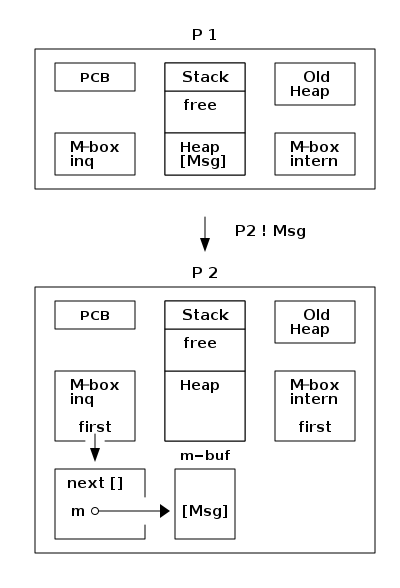
After a GC the message will still be in the m-buf. Not until
the message is received and reachable from some other object on
the heap or from the stack will the message be copied to the process
heap during a GC.
3.6.3. Receiving a Message
Erlang supports selective receive, which means that a message that
doesn’t match can be left in the mailbox for a later receive. And the
processes can be suspended with messages in the mailbox when no
message matches. The msg.save field contains a pointer to a pointer
to the next message to look at.
In later chapters we will cover the details of m-bufs and how the
garbage collector handles mailboxes. We will also go through the
details of how receive is implemented in the BEAM
in later chapters.
3.6.4. Tuning Message Passing
With the new message_queue_data flag introduced in Erlang 19 you
can trade memory for execution time in a new way. If the receiving
process is overloaded and holding on to the main lock, it might be
a good strategy to use the off_heap allocation in order to let the
sending process quickly dump the message in an m-buf.
If two processes have a nicely balanced producer consumer behavior where there is no real contention for the process lock then allocation directly on the receivers heap will be faster and use less memory.
If the receiver is backed up and is receiving more messages than it has time to handle, it might actually start using more memory as messages are copied to the heap, and migrated to the old heap. Since unseen messages are considered live, the heap will need to grow and use more memory.
In order to find out which allocation strategy is best for your system
you will need to benchmark and measure the behavior. The first and easiest
test to do is probably to change the default allocation strategy at
the start of the system. The ERTS flag +hmqd sets the default strategy to
either off_heap or on_heap.
If you start Erlang without this flag the default will be on_heap.
By setting up your benchmark so that Erlang is started with
+hmqd off_heap you can test whether the system behaves better or
worse if all processes use off heap allocation.
Then you might want to find bottle neck processes and test switching
allocation strategies for those processes only.
3.7. The Process Dictionary
There is actually one more memory area in a process where Erlang terms can be stored, the Process Dictionary.
The Process Dictionary (PD) is a process local key-value store. One advantage with it is that all keys and values are kept on the heap of the process, so the terms you store do not need to be copied anywhere as with message passing or ETS tables.
We can now update our view of a process with yet another memory area, PD, the process dictionary, as seen in Figure 19:
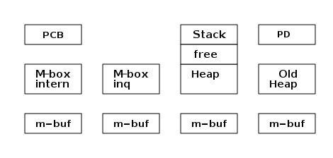
The process dictionary is a very straightforward hash table
implementation. In fact the PD memory area is just the plain bucket array,
and each slot is either NIL (the empty list) if the bucket is empty,
or otherwise it’s a tagged pointer to data on the heap — a simple tuple
{Key, Value} if there is only one entry in the bucket, or a
NIL-terminated list [{Key1, Value1}, …, {KeyN, ValueN}] if the bucket
has N entries. You can find the implementation in the file
erl_process_dict.c.
This way, there is no additional complexity for managing dynamically growing and shrinking bucket lists, and no separate memory management for these data structures apart from the bucket array — it is all handled by the normal creation and freeing of tuples and lists on the heap (which is already as efficient as you’d like). It also means that the garbage collector can easily traverse the hash table much like any Erlang data. (In Chapter 11 we will see the details of how garbage collection works.)
On the downside, the terms in the PD are always live data which needs to be
moved around by the (copying) GC. Hence, storing large amounts of data in
the PD can be a worse choice than using a separate ETS table even if
entries must then be copied in and out — depending on how much load there
is on the GC after the initial growth phase of the dictionary. If you know
you are going to build up a large PD, it can be a good idea to start the
process off with a large initial heap size, as in spawn_opt(…,
[{min_heap_size, Size}]), and then try to do any GC-heavy work in another
process.
Note that, as with any hash table, storing an element in the PD is not completely free — it will result in an extra tuple for the key/value entry and an extra cons cell if the bucket was not empty, which might also cause garbage collection to be triggered. It could also require resizing of the bucket array. Updating an existing key in the dictionary causes the whole list of that bucket to be reallocated to make sure we don’t get pointers from the old heap to the new heap; however, these lists should on average be very short.
3.8. Dig In
In this chapter we have looked at how a process is implemented. In
particular we looked at how the memory of a process is organized, how
message passing works and the information in the PCB. We also looked
at a number of tools for inspecting processes introspection, such as
erlang:process_info/2, and the ETP debug macros.
Use the functions erlang:processes/0 and erlang:process_info/1,2
to inspect the processes in the system. Here are
some functions to try:
1> Ps = erlang:processes().
[<0.0.0>,<0.3.0>,<0.6.0>,<0.7.0>,<0.9.0>,<0.10.0>,<0.11.0>,
 <0.12.0>,<0.13.0>,<0.14.0>,<0.15.0>,<0.16.0>,<0.17.0>,
 <0.19.0>,<0.20.0>,<0.21.0>,<0.22.0>,<0.23.0>,<0.24.0>,
 <0.25.0>,<0.26.0>,<0.27.0>,<0.28.0>,<0.29.0>,<0.33.0>]
2> P = self().
<0.33.0>
3> erlang:process_info(P).
[{current_function,{erl_eval,do_apply,6}},
 {initial_call,{erlang,apply,2}},
 {status,running},
 {message_queue_len,0},
 {messages,[]},
 {links,[<0.27.0>]},
 {dictionary,[]},
 {trap_exit,false},
 {error_handler,error_handler},
 {priority,normal},
 {group_leader,<0.26.0>},
 {total_heap_size,17730},
 {heap_size,6772},
 {stack_size,24},
 {reductions,25944},
 {garbage_collection,[{min_bin_vheap_size,46422},
                      {min_heap_size,233},
                      {fullsweep_after,65535},
                      {minor_gcs,1}]},
 {suspending,[]}]
 4>  lists:keysort(2,[{P,element(2,erlang:process_info(P,
     total_heap_size))} || P <- Ps]).
[{<0.10.0>,233},
 {<0.13.0>,233},
 {<0.14.0>,233},
 {<0.15.0>,233},
 {<0.16.0>,233},
 {<0.17.0>,233},
 {<0.19.0>,233},
 {<0.20.0>,233},
 {<0.21.0>,233},
 {<0.22.0>,233},
 {<0.23.0>,233},
 {<0.25.0>,233},
 {<0.28.0>,233},
 {<0.29.0>,233},
 {<0.6.0>,752},
 {<0.9.0>,752},
 {<0.11.0>,1363},
 {<0.7.0>,1597},
 {<0.0.0>,1974},
 {<0.24.0>,2585},
 {<0.26.0>,6771},
 {<0.12.0>,13544},
 {<0.33.0>,13544},
 {<0.3.0>,15143},
 {<0.27.0>,32875}]
9>
4. The Erlang Type System and Tags
One of the most important aspects of ERTS to understand is how ERTS stores data, that is, how Erlang terms are stored in memory. This gives you the basis for understanding how garbage collection works, how message passing works, and gives you an insight into how much memory is needed.
In this chapter you will learn the basic data types of Erlang and how they are implemented in ERTS. This knowledge will be essential in understanding the chapter on memory allocation and garbage collection, see Chapter 11.
4.1. The Erlang Type System
Erlang is strongly typed. That is, there is no way to coerce one
type into another type, you can only convert from one type to another.
Compare this to e.g. C where you can coerce a char to an int or
any pointer type to a void *.
The Erlang type lattice is quite flat, as you can see in Figure 20. There are only a few real subtypes: numbers have the subtypes integer and float, and list has the subtypes nil and cons. (One could also argue that tuple has one subtype for each size, and similar for maps.)
The Erlang Type Lattice
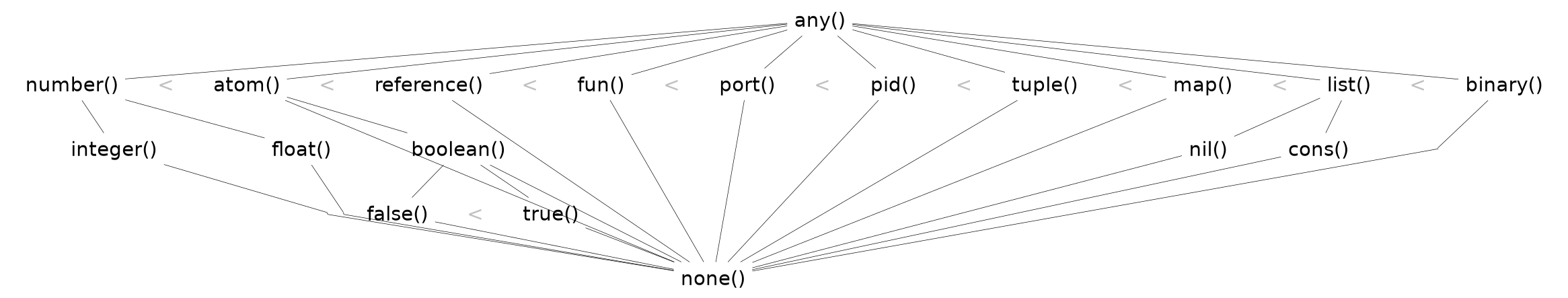
There is a partial order (<, >) on all terms in Erlang where the
types are ordered from left to right in the above lattice.
The order is partial and not total since integers and floats
are converted before comparison. Both 1 < 1.0 and 1.0 < 1 are
false, while 1 =< 1.0, 1 >= 1.0, and 1 == 1.0 are true. The number with
the lesser precision is converted to the number with higher precision.
Usually integers are converted to floats. For very large or small
floats the float is converted to an integer. This happens if all
significant digits are to the left of the decimal point.
For compound structures like tuples and lists, the ordering extends
recursively, so that e.g. {1, 2} < {1, 3} but {2, 1} > {1, 3}. This
means that any set of Erlang terms can be sorted in order, and this
term order is defined by the language.
When two maps are compared for order they are compared as follows: If one map has fewer elements than the other it is considered smaller, just as for tuples. Otherwise the keys are compared in key order, which means all integers are considered smaller than all floats. If all the keys are the same then each value pair (in key order) is compared arithmetically, i.e. by first converting them to the same precision.
The same is true when comparing for equality, thus
#{1 => 1.0} == #{1 => 1} but #{1.0 => 1} /= #{1 => 1}.
Erlang is dynamically typed. That is, types will be checked at runtime and if a type error occurs an exception is thrown. The compiler does not check the types at compile time, unlike in a statically typed language like C or Java where you can get a type error during compilation.
These aspects of the Erlang type system, strongly dynamically typed with an order on the types puts some constraints on the implementation of the language. In order to be able to check and compare types at runtime each Erlang term has to carry its type with it.
This is solved by tagging the terms.
4.2. The Tagging Scheme
In the memory representation of an Erlang term a few bits are reserved for a type tag. For performance reasons the terms are divided into immediates and boxed terms. An immediate term can fit into a machine word, that is, in a register or on a stack slot. A boxed term consists of two parts: a tagged pointer and a number of words stored on the process heap. The boxes stored on the heap have a header and a body, unless it is a list, which is headerless.
Currently ERTS uses a staged tag scheme, the history and reasoning behind the this scheme is explained in a technical report from the HiPE group. (See http://www.it.uu.se/research/publications/reports/2000-029/) The tagging scheme is implemented in erl_term.h.
The basic idea is to use the least significant bits for tags. Since most modern CPU architectures aligns 32- and 64-bit words, there are at least two bits that are "unused" for pointers. These bits can be used as tags instead. Unfortunately those two bits are not enough for all the types in Erlang, more bits are therefore used as needed.
4.2.1. The Primary Tag
The first two bits are called the primary tag, and are used as follows:
  00 Header (on heap) CP (on stack)
  01 List (cons)
  10 Boxed
  11 Immediate
An Immediate (tag 11) is a self-contained word, such as a small integer.
It requires no additional words.
The Boxed tag 10 is used for pointers to objects on the heap,
except lists.
The Header tag 00 is only used on the heap for header words, which we
will explain in Section 4.5. All objects on the heap use a whole number
of machine words, generally starting with a header word.
On the stack, 00 instead indicates a return address or Continuation Pointer — this is a practical choice which means no tagging/untagging of
such pointers needs to be done, since return addresses will always be
word-aligned anyway. This is a better tradeoff than using 00 for
immediates, lists, or boxed values.
The separate List tag (01) is an optimization due to lists being so
heavily used. This lets each cons cell be stored without a header word
on the heap, saving 1/3 of the space otherwise needed for lists, as you
will see in Section 4.3 and Section 4.4.
4.2.2. Immediates
The Immediate tag is further divided like this:
 00 11 Pid
 01 11 Port
 10 11 Immediate 2
 11 11 Small integer
Pids and ports are immediates and can be compared for equality efficiently. They are of course in reality just references, a pid is a process identifier and it points to a process. The process does not reside on the heap of any process but is handled by the PCB. A port works in much the same way.
A PID immediate is packed into a single machine word: the two least
significant bits are the primary tag 11, the next two bits are the
subtype 00, and the remaining high-order bits hold the PID value.
On a 32-bit system those 28 bits are subdivided into a 15-bit process
index (an offset into the process table), a 13-bit serial (to
distinguish reused indices), and a small creation field. When you
print a PID in the shell it appears as <Node.Index.Serial>, where
the creation (Node) disambiguates across restarts. Ports use the same
layout (subtype 01), splitting their high-order bits into a port
number and creation. Because the entire reference lives in one word,
equality (and inequality) tests on PIDs and ports reduce to a single
integer comparison.
There are two types of integers in ERTS, small integers and bignums. Small integers fit in one machine word minus four tag bits, i.e. in 28 or 60 bits for 32 and 64 bits system respectively. Bignums on the other hand can be as large as needed (only limited by the heap space) and are stored on the heap, as boxed objects (see Section 4.5).
By having all four tag bits as ones for small integers the emulator
can make an efficient test when doing integer arithmetic to see if
both arguments are immediates. (is_both_small(x,y) is defined as
(x & y & 1111) == 1111).
The Immediate 2 tag is further divided like this:
 00 10 11 Atom
 01 10 11 Catch
 10 10 11   [UNUSED]
 11 10 11 Nil
Atoms are made up of an index in the atom table and the atom tag. Two atom immediates can be compared for equality by just comparing their immediate representation.
In the atom table atoms are stored as C structs like this:
typedef struct atom {
    IndexSlot slot;  /* MUST BE LOCATED AT TOP OF STRUCT!!! */
    int len;         /* length of atom name */
    int ord0;        /* ordinal value of first 3 bytes + 7 bits */
    byte* name;      /* name of atom */
} Atom;
Thanks to the len and the ord0 fields the order of two atoms can
be compared efficiently as long as they don’t start with the same four
letters.
The Catch immediate is only used on the stack. It contains an indirect pointer to the point in the code where execution should continue after an exception. More on this in Chapter 8.
The Nil tag is used for the empty list written [] in Erlang,
called NIL in the C code. The rest of the word is filled with ones.
4.3. Lists
Lists are made up of
cons cells, which are just two consecutive words on the heap: the head and
the tail (or car and cdr as they are called in LISP, and also in some places in
the ERTS codebase). An empty list is an immediate, as we saw above.
A cons cell could be described by a minimal C struct for building singly linked lists, like this:
struct cons_cell {
    Eterm *head;     /* the value */
    Eterm *tail;     /* the next element */
};
The tail element is usually either another List-tagged pointer to the next
cons cell, or the NIL immediate to mark the end of the list. These are
called proper lists. Erlang is however dynamically typed and the tail
is allowed to be any term, as in [1|2]. These are called improper lists and will be a surprise to any functions that expect a proper list
as input, when they do not find a [] as the last element.
Since each cons cell is identified by the tag in the pointer to the cell,
there is no need for a separate header word, and a cons cell [A|B] thus
uses 33% less memory than a boxed 2-tuple {A,B}. This is also reflected
by a corresponding speed improvement, since only two heap words need to be
initialized rather than three. Therefore, lists are the preferred temporary
data structure for sequences of items.
Note however that for longer term representation of large amounts of data,
lists can use a lot of memory. Suppose you have a million small integers,
each of which could be represented in 2 bytes. On a 64-bit Erlang system,
representing this as a list [1234, 2001, …] would use one million cons
cells each holding a 64-bit immediate integer and a 64-bit pointer to the
next cell in the list, i.e., 16 bytes per cell. That’s 16 megabytes instead
of 2. It would be more space-efficient to pack this data into a binary, but
it all depends on how you need to access these numbers.
4.4. Strings
A string in Erlang (written "…") is just a list of integers
representing Unicode code points. Thus, "XYZ" is syntactical sugar for
[88,89,90]. The Erlang interactive shell will try to detect such lists of
printable characters and show them as strings instead. For example:
Eshell V15.2.2 (press Ctrl+G to abort, type help(). for help)
1> [88,89,90].
"XYZ"| During Erlang’s earlier years, strings were expected to use only Latin-1 (ISO 8859-1) code points. Luckily, these are simply the subset 0-255 of Unicode, so there were few compatibility problems when this range was extended. |
Since allowing the whole Unicode range as "printable characters" would make many lists of assorted integers seem like possible strings, the shell defaults to the Latin-1 range when detecting strings, so for example:
2> [955, 960, 963].
[955,960,963]
just shows the result as a list of numbers, even though 955, 960, and 963
are the Greek letters lambda, pi, and sigma. However, if we start Erlang
with the option +pc unicode, the Erlang shell will be much more generous
with what it considers printable:
$ erl +pc unicode
Erlang/OTP 27 [erts-15.2.2] [source] [64-bit] [smp:8:8] [ds:8:8:10] [async-threads:1] [jit:ns]

Eshell V15.2.2 (press Ctrl+G to abort, type help(). for help)
1> [955, 960, 963].
"λπσ"
Just note that it depends on your console, what encoding it is set to expect, and its available fonts, whether it will be able to actually display those characters.
The string "hello" might then look like this in memory (Figure 21):

This is basically a linked list of UTF-32 encoded characters, and as you can see it wastes quite a lot of memory — especially on a 64-bit machine where it will use 16 bytes per character — compared to the same string as a UTF-8 encoded byte sequence. Therefore, strings are best used as a temporary "text buffer" that you can match on, traverse, and prepend to, and when done you can convert them to UTF-8 encoded Binaries for storing, sending or printing. (We will talk more about Binaries below.)
When Erlang strings get serialized for sending to another node or
storing in ETS tables or on disk, this is done using the Erlang External Term Format, via term_to_binary(). This uses a much more compact
byte encoding for strings. You should generally not need to worry about
strings in those cases — it’s the on-heap representation that you should
avoid hanging on to.
|
4.4.1. IO Lists
IO lists extend erlang strings by allowing binaries, nested lists, strings, and integers to be concatenated without flattening. Each element is either a binary chunk or a list node, and the driver outputs them in sequence with minimal copying.
4.5. Boxed Terms
All other terms on the heap start with a header word. The header word uses a four bit subtag and the primary tag 00. The remaining bits encode the arity which says how many additional words the boxed term uses:
aaaaaaaa...aaaaaaaaaaaaaaaa tttt 00
The subtags are:
 0000 00  ARITYVAL (Tuples)
 0001 00  BINARY_AGGREGATE                |
 001s 00  BIGNUM with sign bit            |
 0100 00  REF                             |
 0101 00  FUN                             | THINGS
 0110 00  FLONUM                          |
 0111 00  EXPORT                          |
 1000 00  REFC_BINARY     |               |
 1001 00  HEAP_BINARY     | BINARIES      |
 1010 00  SUB_BINARY      |               |
 1011 00    [UNUSED]
 1100 00  EXTERNAL_PID  |                 |
 1101 00  EXTERNAL_PORT | EXTERNAL THINGS |
 1110 00  EXTERNAL_REF  |                 |
 1111 00  MAP
4.5.1. Tuples
Tuples (known as ARITYVAL in the ERTS code base) are
simply stored with the header containing the tag and the number of
elements, with the tuple elements (if any) in the following words. For
example, a 5-tuple {$h, $e, $l, $l, $o}` will look like this in memory
(Figure 22)

Note that this means that the empty tuple {} is represented on the heap
by a single word with all bits 0 (arity 0, subtag 0000, and primary tag
00). However, it also requires the boxed pointer to the word on the heap,
so it is not as cheap as NIL which is an immediate and can e.g. be kept
in a register or stored as the tail of a list without needing an additional
heap word.
4.5.2. Binaries
A binary is an immutable array of bytes. Internally, there are four types
of representations of binaries. The two types heap binaries
and refc binaries contain binary data. The other two types, sub
binaries and match contexts (the BINARY_AGGREGATE tag) are smaller
references into one of the other two types.
Binaries that are 64 bytes or less can be stored directly on the process heap as heap binaries. Larger binaries are reference counted and the payload is stored outside of the process heap, while a reference to the payload is stored on the process heap in an object called a ProcBin.
| An important point with binaries is that since they simply represent a chunk of bytes, they never refer to other objects, and the garbage collector does not need to inspect the payload. It is therefore possible to use a different storage strategy tailored to them; in particular, reference counting binaries will never run into the problem of circular references. |
  Heap/Refc Binary Header Word (32-bit view)
  +------------------------------------------+
  |  20-bit or 28-bit length/offset field    |
  +----------------+-------------+-----------+
  | subtag (4-bit) | primary tag | padding?  |
+----------------+-------------+-----------+-
primary tag
00indicates a boxed term header. -
subtag
1001marks a heap binary (payload on heap). -
subtag
1000marks a reference-counted binary (ProcBin).
Following the header:
-
For heap binaries, the binary payload bytes follow immediately.
-
For refc binaries, the header is followed by a ProcBin struct.
Sub binaries (subtag 1010) are views into an existing binary.
They store a header word with length and offset fields, followed by two
machine words. This avoids copying payload data when slicing or matching parts of a binary.
Match contexts (subtag 0001, BINARY_AGGREGATE) are used by the
binary pattern-matching engine. They reference segments of one or more
enclosing binaries without allocating new payload space:
-
They contain a header word with the total number of segments.
-
They include an array of
{pointer, length}tuples pointing into the original binaries.
This allows efficient iteration without flattening or copying data.
We will talk more about binaries in Chapter 11.
4.5.3. Bignums
Any integer too large to fit into a small immediate (word size minus four tag bits) is represented as a bignum, which is a boxed term whose header word encodes both its sign and the number of “limb” words that follow. The header’s primary tag (00) marks it as a heap‐allocated header, the four‐bit subtag (001) identifies it as a bignum, and the highest bit of that subtag carries the sign (0 = positive, 1 = negative). Each subsequent limb is a full machine word holding a slice of the integer in base 2^D_EXP (typically 28 bits on 32-bit builds, 60 bits on 64-bit builds), arranged little-endian (least significant limb first).
Multi-precision arithmetic operates directly on these limb arrays. Addition and subtraction are implemented by scanning limbs word-by-word with carry or borrow propagation (I_add/I_sub), emitting a result limb array whose length may grow by one if there is a final carry. Multiplication uses either the quadratic schoolbook algorithm (I_mul) for small limb counts or the Karatsuba divide-and-conquer method (I_mul_karatsuba) when operand lengths exceed a threshold, with intermediate double-precision products split into high and low halves. Division and remainder use Knuth’s Algorithm D (I_div/I_rem) to compute quotient and remainder limb arrays, adjusting the result sign according to operand signs.
Internally each limb is an ErtsDigit, and you access the limb array of a bignum via the BIG_V(xp) macro, which yields an ErtsDigit* pointer to the least significant word. Individual limbs are read or written with BIG_DIGIT(xp, i) (0-based index, little-endian). All of the core routines in big.c—for instance, I_add, I_sub, I_mul, I_mul_karatsuba, I_div, and I_rem—operate directly on these ErtsDigit* arrays, handling carry/borrow, multi-precision multiplies, and long-division steps. Once the result digits are computed, big_norm recomputes the boxed header (tag, arity, sign) and may even reintegrate the result as a small immediate if it fits in the tag bits.
| While bignums resemble binaries in that they both are just “chunks of bytes”, bignums are always stored on the heap in their entirety, and having a heap full of very large bignums means the garbage collector will need to copy a lot of live data back and forth. It is therefore not such a clever hack to encode a big chunk of binary data as a bignum even if it can be done. [2] |
4.5.4. References
A reference is a “unique” term, often used to tag messages in order
to basically implement a channel over a process mailbox. A reference
is implemented as an 82 bit counter. After 9671406556917033397649407
calls to make_ref/0, the counter will wrap and start over with ref 0
again. You need a really fast machine to do that many calls to
make_ref within your lifetime — unless you restart the node, in which
case it also will start from 0 again, but then all the old local refs
are gone. If you send the ref to another node it becomes an external
ref, see below.
On a 32-bit system a local ref takes up four 32-bit words on the heap. On a 64-bit system a ref takes up three 64-bit words on the heap.
    |00000000 00000000 00000000 11010000| Arity 3 + ref tag
    |00000000 000000rr rrrrrrrr rrrrrrrr| Data0
    |rrrrrrrr rrrrrrrr rrrrrrrr rrrrrrrr| Data1
    |rrrrrrrr rrrrrrrr rrrrrrrr rrrrrrrr| Data2
The reference number is (Data2 bsl 50) + (Data1 bsl 18) + Data0.
4.5.5. Floats
Erlang floats are boxed heap terms tagged with the FLONUM subtag. Each float occupies two machine words: a header word (primary tag 00, subtag 0110) and a 64-bit IEEE 754 payload word. The emulator treats floats as opaque “boxed” values for garbage-collection and comparison, using native CPU instructions for arithmetic when available, and falling back to software routines otherwise.
4.5.6. Records
Records are a compile-time convenience built on tuples: a record of arity N is simply an N-element tuple with the first element an atom naming the record. Access and update macros translate into fixed-index tuple lookups or setelement/3 calls. Because the tuple header (primary tag 00, subtag 0000) encodes the arity, record size and field offsets are known at runtime without extra metadata.
4.6. Conclusion
In this chapter we have explored how Erlang’s dynamic type system is implemented in the ERTS, covering the tagging scheme that unifies immediates and boxed terms for efficient runtime type checks and comparisons. We saw how the underlying tag bits and heap layouts reflect Erlang’s strong yet dynamic typing model. Understanding these encodings will make it easier to grasp the later chapters on memory allocation and garbage collection, where we will examine how boxed terms are managed on the process heap.
5. The Erlang Virtual Machine: BEAM
BEAM (Bogdan’s/Björn’s Abstract Machine) is the machine that executes the code in the Erlang Runtime System. It is a garbage collecting, reduction counting, virtual, non-preemptive, direct threaded, register machine. If that doesn’t tell you much, don’t worry, in the following sections we will go through what each of those words means in this context.
The virtual machine, BEAM, is at the heart of the Erlang node. It is the BEAM that executes the Erlang code. That is, it is BEAM that executes your application code. Understanding how BEAM executes the code is vital to be able to profile and tune your code.
The BEAM design influences large parts of the rest of ERTS. The primitives for scheduling influences the Scheduler (Chapter 10), the representation of Erlang terms (Chapter 4) and the interaction with the memory influences the Garbage Collector (Chapter 12). By understanding the basic design of BEAM you will more easily understand the implementations of these other components.
5.1. Working Memory: A stack machine, it is not
As opposed to its predecessor JAM (Joe’s Abstract Machine) which was a stack machine, the BEAM is a register machine loosely based on WAM [Warren]. In a stack machine each operand to an instruction is first pushed to the working stack, then the instruction pops its operands and then it pushes the result on the stack.
Stack machines are quite popular among virtual machine and programming language implementers since they are quite easy to generate code for, and the code becomes very compact. The compiler does not need to do any register allocation, and most operations do not need any operands (in the instruction stream).
Compiling the expression "8 + 17 * 2." to a stack machine could yield code like:
push 8
push 17
push 2
multiply
add
This code can be generated directly from the parse tree of
the expression. By using Erlang expression and the modules
erl_scan and
erl_parse we
can build the world’s most simplistic compiler:
compile(String) ->
    [ParseTree] = element(2,
			  erl_parse:parse_exprs(
			    element(2,
				    erl_scan:string(String)))),
    generate_code(ParseTree).

generate_code({op, _Line, '+', Arg1, Arg2}) ->
    generate_code(Arg1) ++ generate_code(Arg2) ++ [add];
generate_code({op, _Line, '*', Arg1, Arg2}) ->
    generate_code(Arg1) ++ generate_code(Arg2) ++ [multiply];
generate_code({integer, _Line, I}) -> [push, I].
And an even more simplistic virtual stack machine:
interpret(Code) -> interpret(Code, []).

interpret([push, I |Rest], Stack)              -> interpret(Rest, [I|Stack]);
interpret([add     |Rest], [Arg2, Arg1|Stack]) -> interpret(Rest, [Arg1+Arg2|Stack]);
interpret([multiply|Rest], [Arg2, Arg1|Stack]) -> interpret(Rest, [Arg1*Arg2|Stack]);
interpret([],              [Res|_])            -> Res.
And a quick test run gives us the answer:
1> stack_machine:interpret(stack_machine:compile("8 + 17 * 2.")).
42
Great, you have built your first virtual machine! Handling subtraction, division and the rest of the Erlang language is left as an exercise for the reader.
5.1.1. Registers in BEAM
Anyway, the BEAM is not a stack machine, it is a register machine. In a register machine, instruction operands are stored in registers instead of on the stack, and the result of an operation usually ends up in a specific register. In the BEAM, registers are word-sized memory locations called X registers (X0, X1, …), private to the running process.
Most register machines do still have a stack used for passing arguments to functions and saving return addresses. A section of the stack that holds information about a particular function call is called a stack frame, holding the return address, any input arguments and local variables that don’t fit in registers, and any temporarily saved values during calls to subroutines. [3]
The BEAM has a stack where all the entries in a stack frame are uniformly word-sized just like the X registers, and they are therefore simply called Y registers (Y0, Y1, …) — a terminology borrowed from the WAM [Warren]. In other words, when a BEAM instruction refers to Y0, it means slot 0 in the stack frame of the current call,
X registers are general purpose registers but are also used for passing arguments to called functions, and register X0 (sometimes also called R0) is used for the return value. Since these registers are simply memory locations, not hardware registers, they are not such a limited resource as in a real CPU (where even 32 registers is considered a lot). In the BEAM, there are 1024 X registers available, so function arguments never need to be passed on the stack. (However, the current contents of other live X registers must to be saved on the stack in Y registers across a function call, using a “caller saves” convention.)
The X registers are stored in a C array in the BEAM emulator (separate for each scheduler) and they are globally accessible from all functions. The X0 register is cached in a local variable, which gets kept in a physical machine register on most architectures. Since X0 is heavily used, this is an important optimization.
The Y registers are stored in the current stack frame and are only accessible by the executing function. To save a value across a function call, BEAM allocates space for it in the stack frame and then moves the value to the corresponding Y register. Writing to a Y register for which there is no reserved space is not allowed, since that could overwrite the heap.
Except for the X and Y registers, there are a number of special purpose registers in the BEAM:
-
Htop — The top of the heap (
htop) -
E — The top of the stack (
stop) -
I — instruction pointer
-
FP — Frame Pointer (start of current frame)
-
CP — Continuation Pointer, i.e. function return address
-
fcalls — reduction counter
Registers like Htop and E are cached versions of the corresponding fields in the PCB. When the process has used up its time slice, the values get written back to the PCB and another process gets to run. Because of how the BEAM decides to swap out a process for another (using what can be considered a form of cooperative multitasking) (see Section 5.3), there is no need to save and restore all the X registers when this happens — everything that needs saving will be in Y registers at that time.
The Frame Pointer (FP) is not necessarily a “real” BEAM register — it can be calculated from the stack top given that we know the current size of the stack frame. Tracking it separately might however make other things easier in the implementation, and we will treat it here as if it exists, since it simplifies the presentation.
The Continuation Pointer (CP) gets set to the return address when the BEAM executes a call instruction. Instead of pushing the return address directly on the stack, it is kept in the CP, so that a return instruction can just set the new value of I equal to CP and continue executing. This is an optimization based on the fact that on average, half of all calls (not counting tail calls) will be to leaf functions, i.e., functions that do not call any further functions. When calling a leaf function, storing the return address on the stack is unnecessary. Instead, only the non-leaf functions need to save the CP on the stack and restore it before returning.
Figure 23 shows the layout of registers and the stack frame in the BEAM for a function that uses two Y registers and has saved the CP on the stack. The X and Y registers may contain immediates or tagged pointers (see Chapter 4) to the heap, but they never point to stack slots; there are e.g. no tuples stored in a stack frame.
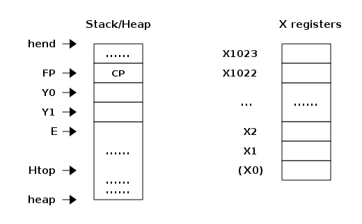
5.1.2. Stack layout example
Let us compile the following program with the 'S' flag:
-module(add).
-export([add/2]).

add(A,B) ->  id(A) + id(B).

id(I) -> I.
Then we get the following code for the add/2 function:
{function, add, 2, 2}.
  {label,1}.
    {line,[{location,"add.erl",4}]}.
    {func_info,{atom,add},{atom,add},2}.
  {label,2}.
    {allocate,1,2}.
    {move,{x,1},{y,0}}.
    {call,1,{f,4}}.
    {swap,{y,0},{x,0}}.
    {call,1,{f,4}}.
    {gc_bif,'+',{f,0},1,[{y,0},{x,0}],{x,0}}.
    {deallocate,1}.
    return.
On entry to the function, the first argument A will be passed in X0, and
the second argument B in X1, by convention.
We can see that the code (starting at label 2) first allocates space for a
single stack slot,[4]
so that Y0 can be used to save the value in X1 over the function
call id(A), which is done by the instruction
{move,{x,1},{y,0}} (read as “move X1 to Y0” or written in imperative style: y0
:= x1).
Argument A is already in X0 (the first argument register), so
the id/1 function at label {f,4} (not shown here) can be called
directly by
{call,1,{f,4}}. (We will come back to what the operand "1" stands for later.)
Then, the result of the call — returned in X0 — needs to be saved on the stack, but the slot Y0 is already occupied by argument
B. Fortunately there is a swap instruction to handle this case, so
we don’t have to use three instructions to first move Y0 to X1, then X0 to
Y0, and then X1 to X0.
Now we have the second argument B in X0, and we can call the id/1
function again by {call,1,{f,4}}. After this, X0 contains id(B) and Y0
contains id(A). We can perform the addition by calling the built-in
function +/2: {gc_bif,'+',{f,0},1,[{y,0},{x,0}],{x,0}}. (We will go
into the details of BIF calls and GC later.) The result is again in X0,
which is where it needs to be for returning from add/2. All that is
needed before the return is to move the stack pointer back again with
a deallocate instruction, and the function is done.
5.2. The BEAM Interpreter
| This section is not about the JIT compiler, which is the newer way of executing BEAM code but which only runs on supported platforms, but about the BEAM instruction interpreter which has been around for much longer and works on all platforms. |
The BEAM interpreter is implemented with a technique called direct threaded code. In this context the word threaded has nothing to do with OS threads, concurrency or parallelism. It is the execution path which is threaded through the virtual machine itself.
5.2.1. Bytecode emulation
If we take a look at our naive stack machine for arithmetic expressions we see that we use Erlang atoms and pattern matching to select which instruction to execute. This is a very heavy machinery to just decode machine instructions. In a real machine implementation we would code each instruction as a "machine word" integer or even a single byte.
We can rewrite our stack machine to be a byte code machine implemented in C. First we rewrite our simple compiler so that it produces byte codes. This is straightforward, just replacing each instruction encoded as an atom with a byte representing the instruction (see below). To be able to handle integers larger than 255 we encode integers with a size byte followed by the integer encoded in bytes.
compile(Expression, FileName) ->
    [ParseTree] = element(2,
			  erl_parse:parse_exprs(
			    element(2,
				    erl_scan:string(Expression)))),
    file:write_file(FileName, generate_code(ParseTree) ++ [stop()]).

generate_code({op, _Line, '+', Arg1, Arg2}) ->
    generate_code(Arg1) ++ generate_code(Arg2) ++ [add()];
generate_code({op, _Line, '*', Arg1, Arg2}) ->
    generate_code(Arg1) ++ generate_code(Arg2) ++ [multiply()];
generate_code({integer, _Line, I}) -> [push(), integer(I)].

stop()     -> 0.
add()      -> 1.
multiply() -> 2.
push()     -> 3.
integer(I) ->
    L = binary_to_list(binary:encode_unsigned(I)),
    [length(L) | L].
Now lets write a simple virtual machine and bytecode interpreter in C. (The full code can be found in the online appendix.)
#define STOP 0
#define ADD  1
#define MUL  2
#define PUSH 3

#define pop()   (stack[--sp])
#define push(X) (stack[sp++] = X)

int run(char *code) {
  int stack[1000];
  int sp = 0, size = 0, val = 0;
  char *ip = code;

  while (*ip != STOP) {
    switch (*ip++) {
    case ADD: push(pop() + pop()); break;
    case MUL: push(pop() * pop()); break;
    case PUSH:
      size = *ip++;
      val = 0;
      while (size--) { val = val * 256 + *ip++; }
      push(val);
      break;
    }
  }
  return pop();
}
As you see, a virtual machine written in C does not need to
be very complicated. This machine is just a loop, checking
the byte code at each instruction by looking at the value
pointed to by the instruction pointer (ip).
For each byte code instruction it will switch on the instruction byte
code and jump to the case which executes the instruction. This
requires a decoding of the instruction and then a jump to the correct
code. If we look at the assembly for vsm.c (gcc -S vsm.c) we see
the inner loop of the decoder:
L11:
        movl    -16(%ebp), %eax
        movzbl  (%eax), %eax
        movsbl  %al, %eax
        addl    $1, -16(%ebp)
        cmpl    $2, %eax
        je      L7
        cmpl    $3, %eax
        je      L8
        cmpl    $1, %eax
        jne     L5
It has to compare the byte code with each instruction code and then do a conditional jump. In a real machine with many instructions this can become quite expensive.
5.2.2. Threaded Code
A better solution would be to have a table with the address of the code — then we could just use an index into the table to load the address and jump without the need to do any comparisons. This technique is sometimes called token threaded code. Taking this a step further we can actually store the address of the code snippet implementing the instruction as the “instruction” itself in the code memory. We could then let the interpreter loop read the next address instead of a single byte, call the routine at that address, and when it returns just advance to the next address. This is called subroutine threaded code. Note however that the code takes up much more space — one whole word per instruction instead of a single byte — but the speed advantage usually makes it worth it on hardware with plenty of memory. (Token threaded code is often used where memory is tight and speed might be less important.)
This approach will make the execution simpler at runtime, but it makes the VM more complicated by requiring a loader. The loader replaces the byte code instructions with addresses to the functions implementing the instructions.
A loader might look like this:
typedef void (*instructionp_t)(void);

void add()  { int x,y; x = pop(); y = pop(); push(x + y); }
void mul()  { int x,y; x = pop(); y = pop(); push(x * y); }
void pushi(){ int x;   x = (int)*ip++;       push(x); }
void stop() { running = 0; }

instructionp_t *read_file(char *name) {
  FILE *file;
  instructionp_t *code;
  instructionp_t *cp;
  long  size;
  char ch;
  unsigned int val;

  file = fopen(name, "r");

  if(file == NULL) exit(1);

  fseek(file, 0L, SEEK_END);
  size = ftell(file);
  code = calloc(size, sizeof(instructionp_t));
  if(code == NULL) exit(1);
  cp = code;

  fseek(file, 0L, SEEK_SET);
  while ( ( ch = fgetc(file) ) != EOF )
    {
      switch (ch) {
      case ADD: *cp++ = &add; break;
      case MUL: *cp++ = &mul; break;
      case PUSH:
	*cp++ = &pushi;
	ch = fgetc(file);
	val = 0;
	while (ch--) { val = val * 256 + fgetc(file); }
	*cp++ = (instructionp_t) val;
	break;
      }
    }
  *cp = &stop;

  fclose(file);
  return code;
}
As we can see, we do more work at load time here, including the decoding of integers larger than 255. (Yes, I know, the code is not safe for very large integers.)
The decode and dispatch loop of the VM becomes quite simple though:
int run() {
  sp = 0;
  running = 1;

  while (running) (*ip++)();

  return pop();
}
Finally, instead of letting each instruction snippet be a function that returns, we can write the code so that each snippet ends with the same small piece of code that the main loop would use to read the next instruction and jump to it. This way, there is no bouncing back and forth between the main loop and the snippets — in fact, the main loop disappears, and each instruction snippet becomes individually responsible for ensuring that it continues to the next instruction. This technique is called direct threaded code. In order to implement this in C, BEAM uses the GCC extension “labels as values”.
5.2.3. The Real BEAM
We will look closer at the BEAM emulator later but for now we will take a
quick look at how the actual BEAM add instruction is implemented. The code is
somewhat hard to follow due to the heavy usage of macros. The
STORE_ARITH_RESULT macro actually hides the dispatch function which
looks something like: I += 4; Goto(*I);.
#define OpCase(OpCode)    lb_##OpCode
#define Goto(Rel) goto *(Rel)

...

 OpCase(i_plus_jId):
 {
     Eterm result;

     if (is_both_small(tmp_arg1, tmp_arg2)) {
	 Sint i = signed_val(tmp_arg1) + signed_val(tmp_arg2);
	 ASSERT(MY_IS_SSMALL(i) == IS_SSMALL(i));
	 if (MY_IS_SSMALL(i)) {
	     result = make_small(i);
	     STORE_ARITH_RESULT(result);
	 }

     }
     arith_func = ARITH_FUNC(mixed_plus);
     goto do_big_arith2;
 }
To make it a little easier to understand how the BEAM dispatcher is implemented, let us take a somewhat imaginary example. We will start with some real external BEAM code, but then I will invent some internal BEAM instructions and implement them in C.
If we start with a simple add function in Erlang:
add(A,B) -> id(A) + id(B).Compiled to BEAM code this will look as follows (or would, before the
swap instruction was added — see Section 5.1.2):
{function, add, 2, 2}.
  {label,1}.
    {func_info,{atom,add},{atom,add},2}.
  {label,2}.
    {allocate,1,2}.
    {move,{x,1},{y,0}}.
    {call,1,{f,4}}.
    {move,{x,0},{x,1}}.
    {move,{y,0},{x,0}}.
    {move,{x,1},{y,0}}.
    {call,1,{f,4}}.
    {gc_bif,'+',{f,0},1,[{y,0},{x,0}],{x,0}}.
    {deallocate,1}.
    return.
(See add.erl and add.S in the online appendix for the full code.)
Now if we zoom in on the three instructions between the function calls in this code:
    {move,{x,0},{x,1}}.
    {move,{y,0},{x,0}}.
    {move,{x,1},{y,0}}.
This code first moves the return value of the function call (x0) to
register x1. Then it moves the previously saved B from the stack slot
y0 into the first argument register (x0). Finally it moves the value in
x1 to the stack slot (y0) so that it will survive the next function
call.
Imagine that we would implement three instruction in BEAM called move_xx,
move_yx, and move_xy (These instructions do not exist in the real BEAM
at the time of this writing — we just use them to illustrate this
example):
#define OpCase(OpCode)    lb_##OpCode
#define Goto(Rel) goto *((void *)Rel)
#define Arg(N) (Eterm *) I[(N)+1]

  OpCase(move_xx):
  {
     x(Arg(1)) = x(Arg(0));
     I += 3;
     Goto(*I);
  }

  OpCase(move_yx): {
    x(Arg(1)) = y(Arg(0));
    I += 3;
    Goto(*I);
  }

  OpCase(move_xy): {
    y(Arg(1)) = x(Arg(0));
    I += 3;
    Goto(*I);
  }
Note that the star in goto * does not mean dereference, the
expression means jump to an address pointer, we should really write it
as goto*.
Now imagine that the compiled C code for these instructions ends up at
memory addresses 0x3000, 0x3100, and 0x3200. When the BEAM code is
loaded, the three move instructions in the code will be replaced by the
memory addresses of the implementation of the instructions. Imagine
that the code ({move,{x,0},{x,1}}, {move,{y,0},{x,0}},
{move,{x,1},{y,0}}) is loaded at address 0x1000:
                    / 0x1000: 0x3000 -> 0x3000: OpCase(move_xx): x(Arg(1)) = x(Arg(0))
{move,{x,0},{x,1}} {  0x1004: 0x0                                I += 3;
                    \ 0x1008: 0x1                                Goto(*I);
                    / 0x100c: 0x3100
{move,{y,0},{x,0}} {  0x1010: 0x0
                    \ 0x1014: 0x0
                    / 0x1018: 0x3200
{move,{x,1},{y,0}} {  0x101c: 0x1
                    \ 0x1020: 0x0
The word at address 0x1000 points to the implementation of
the move_xx instruction. If the register I contains the instruction
pointer, pointing to 0x1000, then the dispatch will be to fetch *I
(i.e. 0x3000) and jump to that address (goto* *I).
In Chapter 7 we will look more closely at some real BEAM instructions and how they are implemented.
5.3. Process Switching
Most modern multi-threading operating systems use preemptive scheduling. This means that the operating system decides when to switch from one process to another, regardless of what the process is doing, typically via interrupts. This protects the other processes from a process misbehaving by not yielding in time.
In cooperative multitasking which uses a non-preemptive scheduler, the running process decides when to yield. This has the disadvantage that a misbehaving process can lock up the CPU so that no other process gets to run (just like in old versions of Microsoft Windows and Mac OS, or in single threaded languages like JavaScript using async/await for concurrency).
On the other hand it has the advantage that a yielding process can decide to only yield in a known state. For example, in a language such as Erlang with dynamic memory management and tagged values, an implementation may be designed such that a process only yields when there are no untagged values in working memory, and no dangling pointers or uninitialized memory addresses.
Take the add instruction as an example: To add two Erlang integers, the emulator first has to untag the integers, then add them together and then tag the result as an integer. If a fully preemptive scheduler is used there would be no guarantee that the process isn’t suspended while the integers are untagged. Or the process could be suspended while it is creating a tuple on the heap, leaving us with half a tuple. This would make it very hard to traverse the stack and heap of a suspended process.
On the language level, all processes are running concurrently and the programmer should not have to deal with explicit yields. BEAM solves this by keeping track of how long a process has been running. This is done by counting reductions. The term originally comes from the mathematical term beta-reduction used in lambda calculus.
The definition of a reduction in BEAM is not very specific, but we can see it as a “small piece of work, which shouldn’t take too long”. Each function call is counted as one reduction. BEAM does a test upon entry to each function to check whether the process has used up all its reductions or not. If there are reductions left, the function gets executed, otherwise the process is suspended and the scheduler picks another ready process to run for a certain number of reductions called a time slice. You can see this as cooperative multitasking but implemented by the compiler, making sure that all programs are well behaved.
Since there are no direct loops in Erlang, only tail-recursive function calls, it is very hard to write a program that does any significant amount of work without using up its reductions.
|
If you write your own NIFs, make sure they can yield and that they bump the reduction counter by an amount proportional to their run time. |
We will go through the details of how the scheduler works in Chapter 10.
5.4. Memory Management
Erlang is a garbage collected language; as an Erlang programmer you do not need to do explicit memory management. On the BEAM code level, though, the code is responsible for initializing data structures, checking for stack and heap overrun, and for allocating enough space on the stack and the heap. If it does not do this correctly, it can result in a crash.
The BEAM instruction test_heap
will ensure that there is as much
space on the heap as requested. If needed the instruction will call
the garbage collector to reclaim space on the heap. The garbage
collector in turn will call the lower levels of the memory subsystem
to allocate or free memory as needed. We will look at the details
of memory management and garbage collection in Chapter 11.
5.5. BEAM: it is virtually unreal
The BEAM is a virtual machine, by which we mean that it is implemented in software instead of in hardware. There have been projects to implement the BEAM by FPGA, and there is nothing stopping anyone from implementing the BEAM in hardware. A better description might be to call the BEAM an Abstract Machine, and see it as blueprint for a machine which can execute BEAM code. And, in fact, the "AM" in BEAM stands for "Abstract Machine".
In this book we will make no distinction between abstract machines, and virtual machines or their implementation. In a more formal setting an abstract machine is a theoretical model of a computer, and a virtual machine is either a software implementation of an abstract machine or a software emulator of a real physical machine.
Unfortunately there exists no official specification of the BEAM — it is currently only defined by the implementation in Erlang/OTP. If you want to implement your own BEAM you would have to try to mimic the current implementation not knowing which parts are essential and which parts are accidental. You would have to mimic every observable behavior to be sure that you have a valid BEAM interpreter.
6. Modules and The BEAM File Format
6.1. Modules
In Erlang, a module is a file containing Erlang functions. It provides a way to group related functions together and use them in other modules. Code loading in Erlang is the process of loading compiled Erlang modules into the BEAM virtual machine. This can be done statically at startup or dynamically while the system is running.
Erlang supports hot code loading, which means you can update a module while your system is running without stopping or restarting the system. This is very convenient during development and debugging. Depending on how you deploy your system it can also be useful when maintaining and running a 24/7 system by allowing you to upgrade a module without stopping the system.
When new code is loaded, the old version remains in memory until there are no processes executing it. Once that’s the case, the old code is purged from the system. Note that if you load a third version of a module before the first version has been purged, then the default behavior of the system is to kill any process that references (has a call on the stack) the first version.
You can load a module into the system dynamically using the code:load_file(Module) function. After a new module is loaded then any fully qualified
calls (i.e. Module:function), also called remote calls, will go to the
new version. Note that if you have a server loop without a remote call
then it will continue running the old code.
The code server is a part of the BEAM virtual machine responsible for managing loaded modules and their code.
Erlang’s distribution model and hot code loading feature make it possible to update code across multiple nodes in a distributed system. However, it’s a complex task that requires careful coordination.
6.2. The BEAM File Format
The definite source of information about the beam file format is obviously the source code of beam_lib.erl (see https://github.com/erlang/otp/blob/maint/lib/stdlib/src/beam_lib.erl). There is actually also a more readable but slightly dated description of the format written by the main developer and maintainer of Beam (see http://www.erlang.se/~bjorn/beam_file_format.html).
The beam file format is based on the interchange file format (EA IFF)#, with two small changes. We will get to those shortly. An IFF file starts with a header followed by a number of “chunks”. There are a number of standard chunk types in the IFF specification dealing mainly with images and music. But the IFF standard also lets you specify your own named chunks, and this is what BEAM does.
| Beam files differ from standard IFF files, in that each chunk is aligned on 4-byte boundary (i.e. 32 bit word) instead of on a 2-byte boundary as in the IFF standard. To indicate that this is not a standard IFF file the IFF header is tagged with “FOR1” instead of “FOR”. The IFF specification suggests this tag for future extensions. |
Beam uses form type “BEAM”. A beam file header has the following layout:
BEAMHeader = <<
  IffHeader:4/unit:8 = "FOR1",
  Size:32/big,                  // big endian, how many more bytes are there
  FormType:4/unit:8 = "BEAM"
>>
After the header multiple chunks can be found. Size of each chunk is aligned to the multiple of 4 and each chunk has its own header (below).
| The alignment is important for some platforms, where unaligned memory byte access would create a hardware exception (named SIGBUS in Linux). This can turn out to be a performance hit or the exception could crash the VM. |
BEAMChunk = <<
  ChunkName:4/unit:8,           // "Code", "Atom", "StrT", "LitT", ...
  ChunkSize:32/big,
  ChunkData:ChunkSize/unit:8,   // data format is defined by ChunkName
  Padding4:0..3/unit:8
>>
This file format prepends all areas with the size of the following area making it easy to parse the file directly while reading it from disk. To illustrate the structure and content of beam files, we will write a small program that extract all the chunks from a beam file. To make this program as simple and readable as possible we will not parse the file while reading, instead we load the whole file in memory as a binary, and then parse each chunk. The first step is to get a list of all chunks:
-module(beamfile1).
-export([read/1]).

read(Filename) ->
   {ok, File} = file:read_file(Filename),
   <<"FOR1",
     Size:32/integer,
     "BEAM",
     Chunks/binary>> = File,
   {Size, read_chunks(Chunks, [])}.

read_chunks(<<N,A,M,E, Size:32/integer, Tail/binary>>, Acc) ->
   %% Align each chunk on even 4 bytes
   ChunkLength = align_by_four(Size),
   <<Chunk:ChunkLength/binary, Rest/binary>> = Tail,
   read_chunks(Rest, [{[N,A,M,E], Size, Chunk}|Acc]);
read_chunks(<<>>, Acc) -> lists:reverse(Acc).

align_by_four(N) -> (4 * ((N+3) div 4)).
A sample run might look like:
> beamfile1:read("beamfile1.beam").
{1116, [{"AtU8",127,
 <<0,0,0,16,9,98,101,97,109,102,105,108,101,49,4,114,101,
 97,100,4,102,105,108,...>>}, {"Code",362,
 <<0,0,0,16,0,0,0,0,0,0,0,178,0,0,0,16,0,0,0,5,1,16,...>>},
 {"StrT",8,<<"FOR1BEAM">>},
 {"ImpT",88,<<0,0,0,7,0,0,0,3,0,0,0,4,0,0,0,1,0,0,0,8,...>>},
 {"ExpT",40,<<0,0,0,3,0,0,0,15,0,0,0,1,0,0,0,15,0,0,0,...>>}, {"Meta",29,
 <<131,108,0,0,0,1,104,2,100,0,16,101,110,97,98,108,101, 100,...>>},
 {"LocT",28,<<0,0,0,2,0,0,0,10,0,0,0,1,0,0,0,11,0,...>>}, {"Attr",40,
 <<131,108,0,0,0,1,104,2,100,0,3,118,115,110,108,0,...>>}, {"CInf",122,
 <<131,108,0,0,0,3,104,2,100,0,7,118,101,114,115,...>>}, {"Dbgi",49,
 <<131,104,3,100,0,13,100,101,98,117,103,95,105,110,...>>},
 {"Line",31,<<0,0,0,0,0,0,0,0,0,0,0,12,0,...>>},
 {"Type",80,<<0,0,0,1,0,0,0,4,31,255,0,0,...>>}]}
Here we can see the chunk names that beam uses.
6.2.1. Atom table chunk
Either the chunk named Atom or the chunk named AtU8 is mandatory. It contains all atoms referred to by the module. For source files with latin1 encoding, the chunk named Atom is used. For utf8 encoded modules, the chunk is named AtU8. The format of the atom chunk is:
AtomChunk = <<
  ChunkName:4/unit:8 = "Atom",
  ChunkSize:32/big,
  NumberOfAtoms:32/big,
  [<<AtomLength:8, AtomName:AtomLength/unit:8>> || repeat NumberOfAtoms],
  Padding4:0..3/unit:8
>>
The format of the AtU8 chunk is the same as above, except that the name of the chunk is AtU8.
| Module name is always stored as the first atom in the table (atom index 0). |
Let us add a decoder for the atom chunk to our Beam file reader:
-module(beamfile2).
-export([read/1]).

read(Filename) ->
   {ok, File} = file:read_file(Filename),
   <<"FOR1",
     Size:32/integer,
     "BEAM",
     Chunks/binary>> = File,
   {Size, parse_chunks(read_chunks(Chunks, []),[])}.

read_chunks(<<N,A,M,E, Size:32/integer, Tail/binary>>, Acc) ->
   %% Align each chunk on even 4 bytes
   ChunkLength = align_by_four(Size),
   <<Chunk:ChunkLength/binary, Rest/binary>> = Tail,
   read_chunks(Rest, [{[N,A,M,E], Size, Chunk}|Acc]);
read_chunks(<<>>, Acc) -> lists:reverse(Acc).

parse_chunks([{"AtU8", _Size,
             <<_Numberofatoms:32/integer, Atoms/binary>>}
            | Rest], Acc) ->
   parse_chunks(Rest,[{atoms,parse_atoms(Atoms)}|Acc]);
parse_chunks([Chunk|Rest], Acc) -> %% Not yet implemented chunk
   parse_chunks(Rest, [Chunk|Acc]);
parse_chunks([],Acc) -> Acc.

parse_atoms(<<Atomlength, Atom:Atomlength/binary, Rest/binary>>) when Atomlength > 0->
   [list_to_atom(binary_to_list(Atom)) | parse_atoms(Rest)];
parse_atoms(_Alignment) -> [].

align_by_four(N) -> (4 * ((N+3) div 4)).
6.2.2. Export table chunk
The chunk named ExpT (for EXPort Table) is mandatory and contains information about which functions are exported.
The format of the export chunk is:
ExportChunk = <<
  ChunkName:4/unit:8 = "ExpT",
  ChunkSize:32/big,
  ExportCount:32/big,
  [ << FunctionName:32/big,
       Arity:32/big,
       Label:32/big
    >> || repeat ExportCount ],
  Padding4:0..3/unit:8
>>
FunctionName is the index in the atom table.
We can extend our parse_chunk function by adding the following clause after the atom handling clause:
parse_chunks([{"ExpT", _Size,
             <<_Numberofentries:32/integer, Exports/binary>>}
            | Rest], Acc) ->
   parse_chunks(Rest,[{exports,parse_exports(Exports)}|Acc]);

...

parse_exports(<<Function:32/integer,
               Arity:32/integer,
               Label:32/integer,
               Rest/binary>>) ->
   [{Function, Arity, Label} | parse_exports(Rest)];
parse_exports(<<>>) -> [].
6.2.3. Import table chunk
The chunk named ImpT (for IMPort Table) is mandatory and contains information about which functions are imported.
The format of the chunk is:
ImportChunk = <<
  ChunkName:4/unit:8 = "ImpT",
  ChunkSize:32/big,
  ImportCount:32/big,
  [ << ModuleName:32/big,
       FunctionName:32/big,
       Arity:32/big
    >> || repeat ImportCount ],
  Padding4:0..3/unit:8
>>
Here ModuleName and FunctionName are indexes in the atom table.
| The code for parsing the import table is similar to that which parses the export table, but not exactly: both are triplets of 32-bit integers, just their meaning is different. See the full code at the end of the chapter. |
6.2.4. Code Chunk
The chunk named Code contains the beam code for the module and is mandatory. The format of the chunk is:
CodeChunk = <<
  ChunkName:4/unit:8 = "Code",
  ChunkSize:32/big,
  SubSize:32/big,
  InstructionSet:32/big,        % Must match code version in the emulator
  OpcodeMax:32/big,
  LabelCount:32/big,
  FunctionCount:32/big,
  Code:(ChunkSize-SubSize)/binary,  % all remaining data
  Padding4:0..3/unit:8
>>
The field SubSize stores the number of words before the code starts. This makes it possible to add new information fields in the code chunk without breaking older loaders.
The InstructionSet field indicates which version of the instruction set the file uses. The version number is increased if any instruction is changed in an incompatible way.
The OpcodeMax field indicates the highest number of any opcode used in the code. New instructions can be added to the system in a way such that older loaders still can load a newer file as long as the instructions used in the file are within the range the loader knows about.
The field LabelCount contains the number of labels so that a loader can preallocate a label table of the right size in one call. The field FunctionCount contains the number of functions so that the functions table could also be preallocated efficiently.
The Code field contains instructions, chained together, where each instruction has the following format:
Instruction = <<
  InstructionCode:8,
  [beam_asm:encode(Argument) || repeat Arity]
>>
Here Arity is hardcoded in the table, which is generated from ops.tab by genop script when the emulator is built from source.
The encoding produced by beam_asm:encode is explained below in the Compact Term Encoding section.
We can parse out the code chunk by adding the following code to our program:
parse_chunks([{"Code", Size, <<SubSize:32/integer,Chunk/binary>>
              } | Rest], Acc) ->
   <<Info:SubSize/binary, Code/binary>> = Chunk,
   %% 8 is size of ChunkSize & SubSize
   OpcodeSize = Size - SubSize - 8,
   <<OpCodes:OpcodeSize/binary, _Align/binary>> = Code,
   parse_chunks(Rest,[{code,parse_code_info(Info), OpCodes}
                      | Acc]);

...

parse_code_info(<<Instructionset:32/integer,
		  OpcodeMax:32/integer,
		  NumberOfLabels:32/integer,
		  NumberOfFunctions:32/integer,
		  Rest/binary>>) ->
   [{instructionset, Instructionset},
    {opcodemax, OpcodeMax},
    {numberoflabels, NumberOfLabels},
    {numberofFunctions, NumberOfFunctions} |
    case Rest of
	 <<>> -> [];
	 _ -> [{newinfo, Rest}]
    end].
We will learn how to decode the beam instructions in a later chapter, aptly named “BEAM Instructions”.
6.2.5. String table chunk
The chunk named StrT is mandatory and contains all constant string literals in the module as one long string. If there are no string literals the chunks should still be present but empty and of size 0.
The format of the chunk is:
StringChunk = <<
  ChunkName:4/unit:8 = "StrT",
  ChunkSize:32/big,
  Data:ChunkSize/binary,
  Padding4:0..3/unit:8
>>
The string chunk can be parsed easily by just turning the string of bytes into a binary:
parse_chunks([{"StrT", _Size, <<Strings/binary>>} | Rest], Acc) ->
    parse_chunks(Rest,[{strings,binary_to_list(Strings)}|Acc]);
6.2.6. Attributes Chunk
The chunk named Attr is optional, but some OTP tools expect the attributes to be present. The release handler expects the "vsn" attribute to be present. You can get the version attribute from a file with: beam_lib:version(Filename), this function assumes that there is an attribute chunk with a "vsn" attribute present.
The format of the chunk is:
AttributesChunk = <<
  ChunkName:4/unit:8 = "Attr",
  ChunkSize:32/big,
  Attributes:ChunkSize/binary,
  Padding4:0..3/unit:8
>>
We can parse the attribute chunk like this:
parse_chunks([{"Attr", Size, Chunk} | Rest], Acc) ->
    <<Bin:Size/binary, _Pad/binary>> = Chunk,
    Attribs = binary_to_term(Bin),
    parse_chunks(Rest,[{attributes,Attribs}|Acc]);
6.2.7. Compilation Information Chunk
The chunk named CInf is optional, but some OTP tools expect the information to be present.
The format of the chunk is:
CompilationInfoChunk = <<
  ChunkName:4/unit:8 = "CInf",
  ChunkSize:32/big,
  Data:ChunkSize/binary,
  Padding4:0..3/unit:8
>>
We can parse the compilation information chunk like this:
parse_chunks([{"CInf", Size, Chunk} | Rest], Acc) ->
    <<Bin:Size/binary, _Pad/binary>> = Chunk,
    CInfo = binary_to_term(Bin),
    parse_chunks(Rest,[{compile_info,CInfo}|Acc]);
6.2.8. Local Function Table Chunk
The chunk named LocT is optional and intended for cross reference tools.
The format is the same as that of the export table:
LocalFunTableChunk = <<
  ChunkName:4/unit:8 = "LocT",
  ChunkSize:32/big,
  FunctionCount:32/big,
  [ << FunctionName:32/big,
       Arity:32/big,
       Label:32/big
    >> || repeat FunctionCount ],
  Padding4:0..3/unit:8
>>| The code for parsing the local function table is basically the same as that for parsing the export and the import table, and we can actually use the same function to parse entries in all tables. See the full code at the end of the chapter. |
6.2.9. Literal Table Chunk
The chunk named LitT is optional and contains all literal values from the module source in compressed form, which are not immediate values. The format of the chunk is:
LiteralTableChunk = <<
  ChunkName:4/unit:8 = "LitT",
  ChunkSize:32/big,
  UncompressedSize:32/big,      % It is nice to know the size to allocate some memory
  CompressedLiterals:ChunkSize/binary,
  Padding4:0..3/unit:8
>>
Where the CompressedLiterals must have exactly UncompressedSize bytes. Each literal in the table is encoded with the External Term Format (erlang:term_to_binary). The format of CompressedLiterals is the following:
CompressedLiterals = <<
  Count:32/big,
  [ <<Size:32/big, Literal:binary>>  || repeat Count ]
>>
The whole table is compressed with zlib:compress/1 (deflate algorithm), and can be uncompressed with zlib:uncompress/1 (inflate algorithm).
We can parse the chunk like this:
parse_chunks([{"LitT", _ChunkSize,
              <<_UnCompressedTableSize:32, Compressed/binary>>}
             | Rest], Acc) ->
    <<_NumLiterals:32,Table/binary>> = zlib:uncompress(Compressed),
    Literals = parse_literals(Table),
    parse_chunks(Rest,[{literals,Literals}|Acc]);

...

parse_literals(<<Size:32,Literal:Size/binary,Tail/binary>>) ->
    [binary_to_term(Literal) | parse_literals(Tail)];
parse_literals(<<>>) -> [].
6.2.10. Abstract Code Chunk
The chunk named Abst is optional and may contain the code in abstract form. If you give the flag debug_info to the compiler it will store the abstract syntax tree for the module in this chunk. OTP tools like the debugger and Xref need the abstract form. The format of the chunk is:
AbstractCodeChunk = <<
  ChunkName:4/unit:8 = "Abst",
  ChunkSize:32/big,
  AbstractCode:ChunkSize/binary,
  Padding4:0..3/unit:8
>>
We can parse the chunk like this
parse_chunks([{"Abst", _ChunkSize, <<>>} | Rest], Acc) ->
    parse_chunks(Rest,Acc);
parse_chunks([{"Abst", _ChunkSize, <<AbstractCode/binary>>} | Rest], Acc) ->
    parse_chunks(Rest,[{abstract_code,binary_to_term(AbstractCode)}|Acc]);
6.2.11. Additional BEAM Chunks
Several new chunks have been added since Erlang OTP 16:
-
Type Chunk (
Type): Introduced in OTP 25, holds simplified type information aiding JIT optimization. -
Function Table Chunk (
FunT): Metadata for anonymous functions (funs). -
Metadata Chunk (
Meta): Holds optional metadata such as documentation or annotations.
The format for the new chunks is:
Type Chunk (Type):
TypeChunk = <<
  ChunkName:4/unit:8 = "Type",
  ChunkSize:32/big,
  Version:32/big,
  Count:32/big,
  TypeData:(Count * 16)/binary,
  Padding4:0..3/unit:8
>>
The Type chunk holds simplified type information used by the JIT compiler
for optimization. Each type entry is a fixed 16-byte record. The data is
not in Erlang external term format, so it cannot be decoded with
binary_to_term. See beam_types.erl in the compiler for the encoding.
Parsing:
parse_chunks([{"Type", _Size, Chunk} | Rest], Acc) ->
    <<_Version:32/big, Count:32/big, TypeData/binary>> = Chunk,
    Types = parse_types(Count, TypeData, []),
parse_chunks(Rest, [{type_info, Types}|Acc]);-
UTF-8 Atom Chunk (
AtU8): Same format as Atom chunk, used when UTF-8 encoding is required:
AtU8Chunk = <<
  ChunkName:4/unit:8 = "AtU8",
  ChunkSize:32/big,
  NumberOfAtoms:32/big,
  [<<AtomLength:8, AtomName:AtomLength/unit:8>> || repeat NumberOfAtoms],
  Padding4:0..3/unit:8
>>-
Function Table (
FunT): Information about local anonymous functions:
FunTableChunk = <<
  ChunkName:4/unit:8 = "FunT",
  ChunkSize:32/big, FunCount:32/big, [<<FunctionName:32/big, Arity:32/big,
      Label:32/big
   >> || repeat FunCount],
  Padding4:0..3/unit:8
>>-
Metadata Chunk (
Meta): Stores metadata like annotations or user-defined properties:
MetaChunk = <<
  ChunkName:4/unit:8 = "Meta",
  ChunkSize:32/big,
  MetaInfo:ChunkSize/binary,
  Padding4:0..3/unit:8
>>
Parsing example:
parse_chunks([{"Meta", Size, Chunk} | Rest], Acc) ->
    <<MetaInfo:Size/binary, _Pad/binary>> = Chunk,
    Meta = binary_to_term(MetaInfo),
    parse_chunks(Rest, [{meta, Meta}|Acc]);
6.2.12. Encryption
Erlang allows for the encryption of debug information in BEAM files. This feature enables developers to keep their source code confidential while still being able to utilize tools such as the Debugger or Xref.
To employ encrypted debug information, a key must be supplied to both the compiler and beam_lib. This key is specified as a string, ideally containing at least 32 characters, including both upper and lower case letters, digits, and special characters.
The default and currently the only type of crypto algorithm used is des3_cbc, which stands for triple DES (Data Encryption Standard) in Cipher Block Chaining mode. The key string is scrambled using erlang:md5/1 to generate the keys used for des3_cbc.
The key can be provided in two ways:
-
Compiler Option: Use the compiler option {debug_info_key,Key} and the function crypto_key_fun/1 to register a function that returns the key whenever beam_lib needs to decrypt the debug information.
-
.erlang.crypt File: If no function is registered, beam_lib searches for an .erlang.crypt file in the current directory, then the user’s home directory, and finally filename:basedir(user_config, "erlang"). If the file is found and contains a key, beam_lib implicitly creates a crypto key function and registers it.
The .erlang.crypt file should contain a list of tuples in the format {debug_info, Mode, Module, Key}. Mode is the type of crypto algorithm (currently only des3_cbc is allowed), Module is either an atom (in which case Key is only used for that module) or [] (in which case Key is used for all modules), and Key is the non-empty key string.
The key in the first tuple where both Mode and Module match is used. It’s important to use unique keys and keep them secure to ensure the safety of the encrypted debug information.
6.2.13. Compression
When you pass the compressed flag to the Erlang compiler, it instructs the compiler to compress the BEAM file that it produces. This can result in a significantly smaller file size, which can be beneficial in environments where disk space is at a premium.
The compressed flag applies zlib compression to the parts of the BEAM file that contain Erlang code and literal data. This does not affect the execution speed of the code, because the code is decompressed when it is loaded into memory, not when it is executed.
To use the compressed flag, you can pass it as an option to the compile function, like so:
compile:file(Module, [compressed]).Or, if you’re using the erlc command-line compiler, you can pass the +compressed option:
erlc +compressed module.erlIt’s important to note that while the compressed flag can reduce the size of the BEAM file, it also increases the time it takes to load the module, because the code must be decompressed. Therefore, it’s a trade-off between disk space and load time.
6.2.14. Compact Term Encoding
Let’s examine the encoding used by beam_asm:encode.
BEAM files use a compact encoding scheme designed to store simple terms
efficiently.
It’s specifically tailored for reducing file size, differing significantly
from the in-memory layout of terms.
After decoding, all encoded values expand into full-sized machine words or
Erlang terms.
Beam_asm is a module in the compiler application, part of the Erlang distribution, it is used to assemble binary content of beam modules.
|
The main goal of this encoding approach is compactness. It efficiently encodes simple terms by packing them into fewer bits. When decoded, these compacted terms expand to standard machine words or Erlang terms.
Here’s the tag format, including recent changes (notably in OTP 20 and OTP 25):

Since OTP 20 this tag format has been changed and the Extended - Float is gone. All following tag values are shifted down by 1: List is 2#10111, fpreg is 2#100111, alloc list is 2#110111 and literal is 2#1010111. Floating point values now go straight to literal area of the BEAM file.
|
It uses the first 3 bits of a first byte to store the tag which defines the type of the following value. If the bits were all 1 (special value 7 or ?tag_z from beam_opcodes.hrl), then a few more bits are used.
For values under 16, the value is placed entirely into bits 4-5-6-7 having bit 3 set to 0:

For values under 2048 (16#800) bit 3 is set to 1, marks that 1 continuation byte will be used and 3 most significant bits of the value will extend into this byte’s bits 5-6-7:

Larger and negative values are first converted to bytes. Then if the value takes 2..8 bytes, bits 3-4 will be set to 1, and bits 5-6-7 will contain the (Bytes-2) size for the value, which follows:

If the following value is greater than 8 bytes, then all bits 3-4-5-6-7 will be set to 1, followed by a nested encoded unsigned literal (macro ?tag_u in beam_opcodes.hrl) value of (Bytes-9):8, and then the data:

Tag Types
When reading compact term format, the resulting integer may be interpreted differently based on what is the value of Tag.
-
For literals the value is index into the literal table.
-
For atoms, the value is atom index MINUS one. If the value is 0, it means
NIL(empty list) instead. -
For labels 0 means invalid value.
-
If tag is character, the value is unsigned unicode codepoint.
-
Tag Extended List contains pairs of terms. Read
Size, create tuple ofSizeand then readSize/2pairs into it. Each pair isValueandLabel.Valueis a term to compare against andLabelis where to jump on match. This is used inselect_valinstruction.
| The addition of type hints allows the compiler and JIT to better cooperate, resulting in more optimized runtime performance in OTP 25 and beyond. |
Refer to beam_asm:encode/2 in the compiler application for details about how this is encoded. Tag values are presented in this section, but also can be found in compiler/src/beam_opcodes.hrl which is generated by beam_makeops.
7. Generic BEAM Instructions
Beam has two different instructions sets, an internal instructions set, called specific, and an external instruction set, called generic.
The generic instruction set is what could be called the official instruction set, this is the set of instructions used by both the compiler and the Beam interpreter. If there was an official Erlang Virtual Machine specification it would specify this instruction set. If you want to write your own compiler to the Beam, this is the instruction set you should target. If you want to write your own EVM this is the instruction set you should handle.
The external instruction set is quite stable, but it does change between Erlang versions, especially between major versions.
This is the instruction set which we will cover in this chapter.
The other instruction set, the specific, is an optimized instruction set used by the Beam to implement the external instruction set. To give you an understanding of how the Beam works we will cover this instruction set in the online appendix. The internal instruction set can change without warning between minor version or even in patch releases. Basing any tool on the internal instruction set is risky.
In this chapter I will go through the general syntax for the instructions and some instruction groups in detail, a complete list of instructions with short descriptions can be found in Appendix B.
7.1. Instruction definitions
The names and opcodes of the generic instructions are defined
in lib/compiler/src/genop.tab.
The file contains a version number for the Beam instruction format, which
also is written to .beam files. This number has so far never changed
and is still at version 0. If the external format would be changed in a
non backwards compatible way this number would be changed.
The file genop.tab is used as input by beam_makeops which is a perl script
which generate code from the ops tabs. The generator is used both to generate
Erlang code for the compiler (beam_opcodes.hrl and beam_opcodes.erl) and to
generate C code for the emulator (beam_opcodes.c and beam_opcodes.h; for
the traditional BEAM interpreter beam_hot.h, beam_warm.h, beam_cold.h are
also generated; and for BeamAsm beamasm_emit.h and beamasm_protos.h are
generated).
Any line in the file starting with "#" is a comment and ignored by
beam_makeops. The file can contain definitions, which turns into a
binding in the perl script, of the form:
NAME=EXPR
Like, e.g.:
BEAM_FORMAT_NUMBER=0
The Beam format number is the same as the instructionset field in
the external beam format. It is only bumped when a backwards
incompatible change to the instruction set is made.
The main content of the file are the opcode definitions of the form:
OPNUM: [-]NAME/ARITY
Where OPNUM and ARITY are integers, NAME is an identifier starting with a lowercase letter (a-z), and :, -, and / are literals.
For example:
1: label/1
The minus sign (-) indicates a deprecated function. A deprecated function keeps its opcode in order for the loader to be sort of backwards compatible (it will recognize deprecated instructions and refuse to load the code).
In the rest of this Chapter we will go through some BEAM instructions in detail. For a full list with brief descriptions see: Appendix B.
7.2. BEAM code listings
As we saw in Chapter 2 we can give the option 'S' to the
Erlang compiler to get a .S file with the BEAM code for the module
in a human and machine readable format (actually as Erlang terms).
Given the file beamexample1.erl:
-module(beamexample1).

-export([id/1]).

id(I) when is_integer(I) -> I.
When compiled with erlc -S beamexample1.erl we get the following
beamexmaple1.S file:
{module, beamexample1}.  %% version = 0

{exports, [{id,1},{module_info,0},{module_info,1}]}.

{attributes, []}.

{labels, 7}.


{function, id, 1, 2}.
  {label,1}.
    {line,[{location,"beamexample1.erl",5}]}.
    {func_info,{atom,beamexample1},{atom,id},1}.
  {label,2}.
    {test,is_integer,{f,1},[{x,0}]}.
    return.


{function, module_info, 0, 4}.
  {label,3}.
    {line,[]}.
    {func_info,{atom,beamexample1},{atom,module_info},0}.
  {label,4}.
    {move,{atom,beamexample1},{x,0}}.
    {line,[]}.
    {call_ext_only,1,{extfunc,erlang,get_module_info,1}}.


{function, module_info, 1, 6}.
  {label,5}.
    {line,[]}.
    {func_info,{atom,beamexample1},{atom,module_info},1}.
  {label,6}.
    {move,{x,0},{x,1}}.
    {move,{atom,beamexample1},{x,0}}.
    {line,[]}.
    {call_ext_only,2,{extfunc,erlang,get_module_info,2}}.
In addition to the actual beam code for the integer identity function we also get some meta instructions.
The first line {module, beamexample1}. %% version = 0 tells
us the module name beamexample1 and the version number for
the instruction set 0.
Then we get a list of exported functions id/1, module_info/0,
module_info/1. As we can see the compiler has added two auto
generated functions to the code. These two functions are just
dispatchers to the generic module info BIFs (erlang:get_module_info/1 and
erlang:get_module_info/2) with the name of the module added as the first
argument.
The line {attributes, []} list all defined compiler attributes, none in
our case.
Then we get to know that there are less than 7 labels in the module,
{labels, 7}, which makes it easy to do code loading in one pass.
The last type of meta instruction is the function instruction on
the format {function, Name, Arity, StartLabel}. As we can see with
the id function the start label is actually the second label in the
code of the function.
The instruction {label, N} is not really an instruction, it does not
take up any space in memory when loaded. It is just to give a local
name (or number) to a position in the code. Each label potentially
marks the beginning of a basic block since it is a potential
destination of a jump.
The first two instructions following the first label ({label,1})
are actually error generating code which adds the line number and
module, function and arity information and throws an exception.
That are the instructions line and func_info.
The meat of the function is after {label,2}, the instruction
{test,is_integer,{f,1},[{x,0}]}. The test instruction tests if its
arguments (in the list at the end, that is variable {x,0} in this
case) fulfills the test, in this case is an integer (is_integer).
If the test succeeds the next instruction (return) is executed.
Otherwise the functions fails to label 1 ({f,1}), that is,
execution continues at label one where a function clause exception
is thrown.
The other two functions in the file are auto generated. If we look at
the second function the instruction {move,{x,0},{x,1}} moves the
argument in register x0 to the second argument register x1. Then the
instruction {move,{atom,beamexample1},{x,0}} moves the module name
atom to the first argument register x0. Finally a tail call is made to
erlang:get_module_info/2
({call_ext_only,2,{extfunc,erlang,get_module_info,2}}). As we will
see in the next section there are several different call instructions.
7.3. Calls
As we will see in Chapter 8, there are several different types
of calls in Erlang. To distinguish between local and remote calls
in the instruction set, remote calls have _ext in their instruction
names. Local calls just have a label in the code of the module, while
remote calls takes a destination of the form {extfunc, Module, Function,
Arity}.
To distinguish between ordinary (stack building) calls and
tail-recursive calls, the latter have either _only or _last in
their name. The variant with _last will also deallocate as many
stack slots as given by the last argument.
There is also a call_fun Arity instruction that calls the closure
stored in register {x, Arity}. The arguments are stored in x0 to {x,
Arity-1}.
For a full listing of all types of call instructions see Appendix B.
7.4. Stack (and Heap) Management
The stack and the heap of an Erlang process on Beam share the same memory area see Chapter 3 and Chapter 11 for a full discussion. The stack grows toward lower addresses and the heap toward higher addresses. Beam will do a garbage collection if more space than what is available is needed on either the stack or the heap.
On entry to a non leaf function the continuation pointer (CP) is saved on
the stack, and on exit it is read back from the stack. This is done by the
allocate and deallocate instructions, which are used for setting up
and tearing down the stack frame for the current instruction.
A function skeleton for a leaf function looks like this:
{function, Name, Arity, StartLabel}.
  {label,L1}.
    {func_info,{atom,Module},{atom,Name},Arity}.
  {label,L2}.
    ...
    return.
A function skeleton for a non leaf function looks like this:
{function, Name, Arity, StartLabel}.
  {label,L1}.
    {func_info,{atom,Module},{atom,Name},Arity}.
  {label,L2}.
    {allocate,Need,Live}.

    ...
    call ...
    ...

    {deallocate,Need}.
    return.
The instruction allocate StackNeed Live saves the continuation
pointer (CP) and allocate space for StackNeed extra words on the
stack. If a GC is needed during allocation save Live number of X
registers. E.g. if Live is 2 then registers x0 and x1 are saved.
When allocating on the stack, the stack pointer (E) is decreased.

For a full listing of all types of allocate and deallocate instructions see Appendix B.
7.5. Message Passing
Sending a message is straight forward in beam code. You just use the
send instruction. Note though that the send instruction does not
take any arguments, it is more like a function call. It assumes that
the arguments (the destination and the message) are in the argument
registers x0 and x1. The message is also copied from x1 to x0.
Receiving a message is a bit more complicated since it involves both selective receive with pattern matching and introduces a yield/resume point within a function body. (There is also a special feature to minimize message queue scanning using refs, more on that later.)
7.5.1. A Minimal Receive Loop
A minimal receive loop, which accepts any message and has no timeout
(e.g. receive _ -> ok end) looks like this in BEAM code:
  {label,1}.
    {loop_rec,{f,2},{x,0}}.
    remove_message.
    {jump,{f,3}}.
  {label,2}.
    {wait,{f,1}}.
  {label,3}.
     ...
The loop_rec L2 x0 instruction first checks if there is any message
in the message queue. If there are no messages execution jumps to L2,
where the process will be suspended waiting for a message to arrive.
If there is a message in the message queue the loop_rec instruction
also moves the message from the m-buf to the process heap. See
Chapter 11 and Chapter 3 for details of the m-buf
handling.
For code like receive _ -> ok end, where we accept any messages,
there is no pattern matching needed, we just do a remove_message
which unlinks the next message from the message queue. (It also
removes any timeout, more on this soon.)
7.5.2. A Selective Receive Loop
For a selective receive like e.g. receive [] -> ok end we will
loop over the message queue to check if any message in the queue
matches.
  {label,1}.
    {loop_rec,{f,3},{x,0}}.
    {test,is_nil,{f,2},[{x,0}]}.
    remove_message.
    {jump,{f,4}}.
  {label,2}.
    {loop_rec_end,{f,1}}.
  {label,3}.
    {wait,{f,1}}.
  {label,4}.
    ...
In this case we do a pattern match for Nil after the loop_rec
instruction if there was a message in the mailbox. If the message
doesn’t match we end up at L2 where the instruction loop_rec_end
advances the save pointer to the next message (p->msg.save =
&(*p->msg.save)->next) and jumps back to L1.
If there are no more messages in the message queue the process is
suspended by the wait instruction at L3 with the save pointer pointing
to the end of the message queue. When the processes is rescheduled
it will only look at new messages in the message queue (after the save
point).
7.5.3. A Receive Loop With a Timeout
If we add a timeout to our selective receive the wait instruction is replaced by a wait_timeout instruction followed by a timeout instruction and the code following the timeout.
  {label,1}.
    {loop_rec,{f,3},{x,0}}.
    {test,is_nil,{f,2},[{x,0}]}.
    remove_message.
    {jump,{f,4}}.
  {label,2}.
    {loop_rec_end,{f,1}}.
  {label,3}.
    {wait_timeout,{f,1},{integer,1000}}.
    timeout.
  {label,4}.
    ...
The wait_timeout instructions sets up a timeout timer with the given
time (1000 ms in our example) and it also saves the address of the
next instruction (the timeout) in p->def_arg_reg[0] and then
when the timer is set, p->i is set to point to def_arg_reg.
This means that if no matching message arrives while the process is suspended a timeout will be triggered after 1 second and execution for the process will continue at the timeout instruction.
Note that if a message that doesn’t match arrives in the mailbox, the
process is scheduled for execution and will run the pattern matching
code in the receive loop, but the timeout will not be canceled. It is
the remove_message code which also removes any timeout timer.
The timeout instruction resets the save point of the mailbox to the
first element in the queue, and clears the timeout flag (F_TIMO) from
the PCB.
7.5.4. The Synchronous Call Trick (aka The Ref Trick)
We have now come to the last version of our receive loop, where we use the ref trick alluded to earlier to avoid a long message box scan.
A common pattern in Erlang code is to implement a type of "remote
call" with send and a receive between two processes. This is for
example used by gen_server. This code is often hidden behind a library
of ordinary function calls. E.g., you call the function
counter:increment(Counter) and behind the scene this turns into
something like Counter ! {self(), inc}, receive {Counter, Count} ->
Count end.
This is usually a nice abstraction to encapsulate state in a process. There is a slight problem though when the mailbox of the calling process has many messages in it. In this case the receive will have to check each message in the mailbox to find out that no message except the last matches the return message.
This can quite often happen if you have a server that receives many messages and for each message does a number of such remote calls, if there is no back throttle in place the servers message queue will fill up.
To remedy this there is a hack in ERTS to recognize this pattern and avoid scanning the whole message queue for the return message.
The compiler recognizes code that uses a newly created reference (ref) in a receive, and emits code to avoid the long inbox scan since the new ref can not already be in the inbox.
  Ref = make_ref(),
  Counter ! {self(), inc, Ref},
  receive
    {Ref, Count} -> Count
  end.
This gives us the following skeleton for a complete receive.
    {recv_mark,{f,3}}.
    {call_ext,0,{extfunc,erlang,make_ref,0}}.
    ...
    send.
    {recv_set,{f,3}}.
  {label,3}.
    {loop_rec,{f,5},{x,0}}.
    {test,is_tuple,{f,4},[{x,0}]}.
    ...
    {test,is_eq_exact,{f,4},[{x,1},{y,0}]}.
    ...
    remove_message.
    ...
    {jump,{f,6}}.
  {label,4}.
    {loop_rec_end,{f,3}}.
  {label,5}.
    {wait,{f,3}}.
  {label,6}.
The recv_mark instruction saves the current position (the end
msg.last) in msg.saved_last and the address of the label
in msg.mark
The recv_set instruction checks that msg.mark points to the next
instruction and in that case moves the save point (msg.save) to the
last message received before the creation of the ref
(msg.saved_last). If the mark is invalid ( i.e. not equal to
msg.save) the instruction does nothing.
8. Different Types of Calls, Linking and Hot Code Loading
Function calls in BEAM can be categorized into different types.
8.1. Local Calls
A local call occurs when a function is invoked within the same module without explicitly specifying the module name. These calls are resolved at compile time and are guaranteed to execute within the same version of the module as the caller.
Example:
foo() -> bar(). % Local call within the same module8.2. Remote Calls
A remote call explicitly specifies the module name, ensuring that the latest loaded version of the module is used.
Example:
foo() -> ?MODULE:bar(). % Remote call ensuring latest module versionRemote calls facilitate hot code loading, enabling live updates to modules without requiring system restarts.
8.3. Code Loading
In the Erlang Runtime System the code loading is handled by the
code server. The code server will call the lower level BIFs in the
erlang module for the actual loading. But the code server also
determines the purging policy.
The runtime system can keep two versions of each module, a current version and an old version. All fully qualified (remote) calls go to the current version. Local calls in the old version and return addresses on the stack can still go to the old version.
If a third version of a module is loaded and there are still processes running (have pointers on the stack to) the code server will kill those processes and purge the old code. Then the current version will become old and the third version will be loaded as the current version.
8.4. Hot Code Loading
As we saw there is not only a syntactic difference but also a semantic difference between a local function call and a remote function call. A remote call, or a "fully quallified call", that is a call to a function in a named module, is guaranteed to go to the latest loaded version of that module. A local call, an unqualified call to a function within the same module, is guaranteed to go to the same version of the code as the caller.
A call to a local function can be turned into a remote call by
specifying the module name at the call site. This is usually
done with the ?MODULE macro as in ?MODULE:foo().
A remote call to a non local module can not be turned into
a local call, i.e. there is no way to guarantee the version
of the callee in the caller.
This is an important feature of Erlang which makes hot code loading or hot upgrades possible. Just make sure you have a remote call somewhere in your server loop and you can then load new code into the system while it is running; when execution reaches the remote call it will switch to executing the new code.
A common way of writing server loops is to have a local call for the main loop and a code upgrade handler which does a remote call and possibly a state upgrade:
loop(State) ->
  receive
    upgrade ->
       %% Force a call to the latest version of the code.
       NewState = ?MODULE:code_upgrade(State),
       ?MODULE:loop(NewState);
     Msg ->
       %% In other cases we call the old version of the code.
       %% That is the version of the code that also handles old data.
       NewState = handle_msg(Msg, State),
       loop(NewState)
   end.
With this construct, which is basically what gen_server uses,
the programmer has control over when and how a code upgrade is done.
The hot code upgrade is one of the most important features of Erlang
which makes it possible to write servers that operates 24/7 year out
and year in. It is also one of the main reasons why Erlang is
dynamically typed. It is very hard in a statically typed language to
give type for the code_upgrade function. (It is also hard to give the
type of the loop function). These types will change in the future as
the type of State changes to handle new features.
For a language implementer concerned with performance, the hot code loading functionality is a burden though. Since each call to or from a remote module can change to new code in the future it is very hard to do whole program optimization across module boundaries. (Hard but not impossible, there are solutions but so far I have not seen one fully implemented).
8.5. Closure Calls
Closures in Erlang allow functions to be passed as values, capturing variables from their defining scope.
Example:
make_adder(N) -> fun(X) -> X + N end.Calling a Closure
Once a closure is created, it can be called like any other function.
Example:
Adder = make_adder(5),
Result = Adder(10). % Returns 15
Passing Closures as Arguments
Closures can be passed to higher-order functions for more flexible behavior.
Example:
apply_fun(F, X) -> F(X).

Result = apply_fun(make_adder(3), 7). % Returns 10
Returning Closures from Functions
Functions can return closures, allowing dynamic function generation.
Example:
make_multiplier(N) -> fun(X) -> X * N end.

Multiplier = make_multiplier(2),
Result = Multiplier(4). % Returns 8
Closures enable dynamic execution and are commonly used in higher-order functions.
8.6. Dynamic Invocation
You can use variables to dynamically invoke functions at runtime.
Example:
M = lists,
F = map,
Result = M:F(fun(X) -> X * 2 end, [1,2,3]).
This dynamic invocation technique is less efficient than direct calls but provides flexibility in selecting execution paths at runtime. This can be used to implement a callback system where the module that exports a specific set of functions and you just pass the module name around. This technique makes it much harder for analytic tools like Dialyzer to find errors in the code since the call graph is not known at compile time.
8.7. Higher-Order Functions and Hot Code Loading
Higher-order functions allow passing behavior dynamically, which interacts uniquely with hot code loading.
Example:
init() ->
  F = ?MODULE:foo/1,
  L = fun(X) -> foo(X) end,
  loop(F, L).

foo(X) -> X + 1.

loop(F, L) ->
  F(1),
  L(2),
  loop(F, L).
Since L is a local function it will always return X + 1. If the module is reloaded and foo/1 is changed to return X + 2 then F will return X + 2. If the module is reloaded twice
then the process will crash since L refers to a purged version of the module.
8.8. Conclusion
Function call efficiency in Erlang follows a clear hierarchy, as outlined in the Efficiency Guide:
Explicit calls, both local and remote (foo(), m:foo()) are the most efficient.
I would like to add that the most efficient call is a local call to a function in the same module. This is because the call can be resolved at compile time and the function can be inlined. This is not possible for a remote call since the module can be changed at runtime.
Even though the JIT compiler can do a good job with remote calls it does not inline them as of OTP 27.
Calling a closure (Fun(), apply(Fun, [])) is slightly slower but still efficient.
Applying a function () (Mod:Name(), apply(Mod, Name, [])) with a known number of arguments at compile time is next in efficiency. (You can not apply a function that is not exported from a module.)
Applying an exported function with an unknown number of arguments (apply(Mod, Name, Args)) is the least efficient.
The Erlang runtime system is optimized for local calls and remote calls to the current version of a module. Hot code loading is a powerful feature that enables live updates to running systems, but it comes with performance trade-offs. It is also important to understand that reloading a module two times will purge the old version of the module and any references to it will crash the process holding the reference.
9. The BEAM Loader
9.1. Transforming from Generic to Specific instructions
The BEAM loader does not just take the external beam format and write it to memory. It also does a number of transformations on the code and translates from the external (generic) format to the internal (specific) format.
The code for the loader can be found in beam_load.c (in
erts/emulator/beam) but most of the logic for the translations are in
the file ops.tab (in the same directory).
The first step of the loader is to parse beam file, basically the same work as we did in Erlang in Chapter 6 but written in C.
Then the rules in ops.tab are applied to instructions in the code chunk to translate the generic instruction to one or more specific instructions.
The translation table works through pattern matching. Each line in the file defines a pattern of one or more generic instructions with arguments and optionally an arrow followed by one or more instructions to translate to.
The transformations in ops tab tries to handle patterns of instructions generated by the compiler and peephole optimize them to fewer specific instructions. The ops tab transformations tries to generate jump tables for patterns of selects.
The file ops.tab is not parsed at runtime, instead a pattern matching
program is generated from ops.tab and stored in an array in a
generated C file. The perl script beam_makeops (in
erts/emulator/utils) generates a target specific set of opcodes and
translation programs in the files beam_opcodes.h and
beam_opcodes.c (these files end up in the given target directory
e.g. erts/emulator/x86_64-unknown-linux-gnu/opt/smp/).
The same program (beam_makeops) also generates the Erlang code for the
compiler back end beam_opcodes.erl.
9.2. Understanding ops.tab
The transformations in
ops.tab
are executed in the order that they are written in the file. So just like in
Erlang pattern matching, the different rules are triggered from top to bottom.
The types that ops.tab uses for arguments in instructions can be found in
Appendix B.
9.2.1. Transformations
Most of the rules in ops.tab are transformations between different
instructions. A simple transformation looks like this:
move S x==0 | return => move_return S
This combines a move from any location to x(0) and return into a single
instruction called move_return. Let’s break the transformation apart to
see what the different parts do.
- move
-
is the instruction that the pattern first has to match. This can be either a generic instruction that the compiler has emitted, or a temporary instruction that
ops.tabhas emitted to help with transformations. - S
-
is a variable binding any type of value. Any value in the pattern (left hand side or
⇒) that is used in the generator (right hand side of⇒) has to be bound to a variable. - x==0
-
is a guard that says that we only apply the transformation if the target location is an
xregister with the value0. It is possible to chain multiple types and also bind a variable here. For instanceD=xy==0would allow bothxandyregisters with a value of0and also bind the argument to the variableD. - |
-
signifies the end of this instruction and the beginning of another instruction that is part of the same pattern.
- return
-
is the second instruction to match in this pattern.
⇒-
signifies the end of the pattern and the start of the code that is to be generated.
- move_return S
-
is the name of the generated instruction together with the name of the variable on the lhs. It is possible to generate multiple instructions as part of a transformation by using the
|symbol.
More complex translations can be done in ops.tab. For instance take the
select_val
instruction. It will be translated by the loader into either a jump table, a linear
search array or a binary search array depending on the input values.
is_integer Fail=f S | select_val S=s Fail=f Size=u Rest=* | \
  use_jump_tab(Size, Rest) => gen_jump_tab(S, Fail, Size, Rest)
The above transformation creates a jump table if possible of the select_val.
There are a bunch of new techniques used in the transformations.
- S
-
is used in both
is_integerandselect_val. This means that both the values have to be of the same type and have the same value. Furthermore theS=sguard limits the type to a be a source register. - Rest=*
-
allows a variable number of arguments in the instruction and binds them to variable
Rest. - use_jump_tab(Size, Rest)
-
calls the use_jump_tab C function in
beam_load.cthat decides whether the arguments in theselect_valcan be transformed into a jump table. - \
-
signifies that the transformation rule continues on the next line.
- gen_jump_tab(S, Fail, Size, Rest)
-
calls the gen_jump_tab C function in
beam_load.cthat takes care of generating the appropriate instruction.
9.2.2. Specific instruction
When all transformations are done, we have to decide how the specific instruction should
look like. Let’s continue to look at move_return:
%macro: move_return MoveReturn -nonext
move_return x
move_return c
move_return n
This will generate three different instructions that will use the
MoveReturn
macro in beam_emu.c to do the work.
- %macro: move_return
-
this tells
ops.tabto generate the code formove_return. If there is no%macroline, the instruction has to be implemented by hand in beam_emu.c. The code for the instruction will be placed inbeam_hot.horbeam_cold.hdepending on if the%hotor%colddirective is active. - MoveReturn
-
tells the code generator to that the name of the c-macro in beam_emu.c to use is MoveReturn. This macro has to be implemented manually.
- -nonext
-
tells the code generator that it should not generate a dispatch to the next instruction, the
MoveReturnmacro will take care of that. - move_return x
-
tells the code generator to generate a specific instruction for when the instruction argument is an x register.
cfor when it is a constant,nwhen it isNIL. No instructions are in this case generated for when the argument is a y register as the compiler will never generate such code.
The resulting code in beam_hot.h will look like this:
OpCase(move_return_c):
    {
    MoveReturn(Arg(0));
    }

OpCase(move_return_n):
    {
    MoveReturn(NIL);
    }

OpCase(move_return_x):
    {
    MoveReturn(xb(Arg(0)));
    }
All the implementer has to do is to define the MoveReturn macro in beam_emu.c and
the instruction is complete.
The %macro rules can take multiple different flags to modify the code that
gets generated.
The examples below assume that there is a specific instructions looking like this:
%macro move_call MoveCall
move_call x f
without any flags to the %macro the following code will be generated:
BeamInstr* next;
PreFetch(2, next);
MoveCall(Arg(0));
NextPF(2, next);| The PreFetch and NextPF macros make sure to load the address to jump to next before the instruction is executed. This trick increases performance on all architectures by a variying amount depending on cache architecture and super scalar properties of the CPU. |
- -nonext
-
Don’t emit a dispatch for this instructions. This is used for instructions that are known to not continue with the next instructions, i.e. return, call, jump.
%macro move_call MoveCall -nonext
MoveCall(xb(Arg(0)));- -arg_*
-
Include the arguments of type * as arguments to the c-macro. Not all argument types are included by default in the c-macro. For instance the type
fused for fail labels and local function calls is not included. So giving the option-arg_fwill include that as an argument to the c-macro.
%macro move_call MoveCall -arg_f
MoveCall(xb(Arg(0)), Arg(1));- -size
-
Include the size of the instruction as an argument to the c-macro.
%macro move_call MoveCall -size
MoveCall(xb(Arg(0)), 2);- -pack
-
Pack any arguments if possible. This places multiple register arguments in the same word if possible. As register arguments can only be 0-1024, we only need 10 bits to store them + 2 for tagging. So on a 32-bit system we can put 2 registers in one word, while on a 64-bit we can put 4 registers in one word. Packing instruction can greatly decrease the memory used for a single instruction. However there is also a small cost to unpack the instruction, which is why it is not enabled for all instructions.
The example with the call cannot do any packing as f cannot be packed and only one
other argument exists. So let’s look at the
put_list
instruction as an example instead.
%macro:put_list PutList -pack
put_list x x x
BeamInstr tmp_packed1;
BeamInstr* next;
PreFetch(1, next);
tmp_packed1 = Arg(0);
PutList(xb(tmp_packed1&BEAM_TIGHT_MASK),
        xb((tmp_packed1>>BEAM_TIGHT_SHIFT)&BEAM_TIGHT_MASK),
        xb((tmp_packed1>>(2*BEAM_TIGHT_SHIFT))));
NextPF(1, next);
This packs the 3 arguments into 1 machine word, which halves the required memory for this instruction.
- -fail_action
-
Include a fail action as an argument to the c-macro. Note that the
ClauseFail()macro assumes the fail label is in the first argument of the instructions, so in order to use this in the above example we should transform themove_call x ftomove_call f x.
%macro move_call MoveCall -fail_action
MoveCall(xb(Arg(0)), ClauseFail());- -gen_dest
-
Include a store function as an argument to the c-macro.
%macro move_call MoveCall -gen_dest
MoveCall(xb(Arg(0)), StoreSimpleDest);- -goto
-
Replace the normal next dispatch with a jump to a c-label inside beam_emu.c
%macro move_call MoveCall -goto:do_call
MoveCall(xb(Arg(0)));
goto do_call;
9.3. Optimizations
The loader performs many peephole optimizations when loading the code. The most important ones are instruction combining and instruction specialization.
Instruction combining is the joining of two or more smaller instructions into one larger instruction. This can lead to a large speed up of the code if the instructions are known to follow each other most of the time. The speed up is achieved because there is no longer any need to do a dispatch in between the instructions, and also the C compiler gets more information to work with when it is optimizing that instruction. When to do instruction combining is a trade-off where one has to consider the impact the increased size of the main emulator loop has vs the gain when the instruction is executed.
Instruction specialization removes the need to decode the arguments in an instruction.
So instead of having one move_sd instruction, move_xx, move_xy etc are generated
with the arguments already decoded. This reduces the decode cost of the instructions,
but again it is a tradeoff vs emulator code size.
9.3.1. select_val optimizations
The select_val instruction is emitted by the compiler to do control flow handling
of many functions or case clauses. For instance:
select(1) -> 3;
select(2) -> 3;
select(_) -> error.
compiles to:
{function, select, 1, 2}.
  {label,1}.
    {line,[{location,"select.erl",5}]}.
    {func_info,{atom,select},{atom,select},1}.
  {label,2}.
    {test,is_integer,{f,4},[{x,0}]}.
    {select_val,{x,0},{f,4},{list,[{integer,2},{f,3},{integer,1},{f,3}]}}.
  {label,3}.
    {move,{integer,3},{x,0}}.
    return.
  {label,4}.
    {move,{atom,error},{x,0}}.
    return.
The values in the condition are only allowed to be either integers
or atoms. If the value is of any other type the compiler will not emit a
select_val instruction. The loader uses a couple of heuristics to figure
out what type algorithm to use when doing the select_val.
- jump_on_val
-
Create a jump table and use the value as the index. This is very efficient and happens when a group of close together integers are used as the value to select on. If not all values are present, the jump table is padded with extra fail label slots.
- select_val2
-
Used when only two values are to be selected upon and they do not fit in a jump table.
- select_val_lins
-
Do a linear search of the sorted atoms or integers. This is used when a small amount of atoms or integers are to be selected from.
- select_val_bins
-
Do a binary search of the sorted atoms or integers.
9.3.2. pre-hashing of literals
When a literal is loaded and used as an argument to any of the bifs or instructions that need a hashed value of the literal, instead of hashing the literal value every time, the hash is created by the loader and used by the instructions.
Examples of code using this technique are maps instructions and the process dictionary bifs.
10. Scheduling
To fully understand where time in an ERTS system is spent you need to understand how the system decides which Erlang code to run and when to run it. These decisions are made by the Scheduler.
The scheduler is responsible for the real-time guarantees of the system. In a strict Computer Science definition of the word real-time, a real-time system has to be able to guarantee a response within a specified time. That is, there are real deadlines and each task has to complete before its deadline. In Erlang there are no such guarantees, a timeout in Erlang is only guaranteed to not trigger before the given deadline.
In a general system like Erlang where we want to be able to handle all sorts of programs and loads, the scheduler will have to make some compromises. There will always be corner cases where a generic scheduler will behave badly. After reading this chapter you will have a deeper understanding of how the Erlang scheduler works and especially when it might not work optimally. You should be able to design your system to avoid the corner cases and you should also be able to analyze a misbehaving system.
10.1. Concurrency, Parallelism, and Preemptive Multitasking
Erlang is a concurrent language. When we say that processes run concurrently we mean that for an outside observer it looks like two processes are executing at the same time. In a single core system this is achieved by preemptive multitasking. This means that one process will run for a while, and then the scheduler of the virtual machine will suspend it and let another process run.
In a multicore or a distributed system we can achieve true parallelism, that is, two or more processes actually executing at the exact same time. In an SMP enabled emulator the system uses several OS threads to indirectly execute Erlang processes by running one scheduler and emulator per thread. In a system using the default settings for ERTS there will be one thread per enabled core (physical or hyper threaded).
We can check that we have a system capable of parallel execution, by checking if SMP support is enabled:
iex(1)> :erlang.system_info :smp_support
true
We can also check how many schedulers we have running in the system:
iex(2)> :erlang.system_info :schedulers_online
4
We can see this information in the Observer as shown in the figure below.
If we spawn more processes than schedulers we have and
let them do some busy work we can see that there are a number
of processes running in parallel and some processes that
are runnable but not currently running. We can see this
with the function erlang:process_info/2.
1> Loop = fun (0, _) -> ok; (N, F) -> F(N-1, F) end,
   BusyFun = fun() -> spawn(fun () -> Loop(1000000, Loop) end) end,
   SpawnThem = fun(N) -> [ BusyFun() || _ <- lists:seq(1, N)] end,
   GetStatus = fun() -> lists:sort([{erlang:process_info(P, [status]), P}
                        || P <- erlang:processes()]) end,
   RunThem = fun (N) -> SpawnThem(N), GetStatus() end,
   RunThem(8).

[{[{status,garbage_collecting}],<0.62.0>},
 {[{status,garbage_collecting}],<0.66.0>},
 {[{status,runnable}],<0.60.0>},
 {[{status,runnable}],<0.61.0>},
 {[{status,runnable}],<0.63.0>},
 {[{status,runnable}],<0.65.0>},
 {[{status,runnable}],<0.67.0>},
 {[{status,running}],<0.58.0>},
 {[{status,running}],<0.64.0>},
 {[{status,waiting}],<0.0.0>},
 {[{status,waiting}],<0.1.0>},

...
We will look closer at the different statuses that a process can have later in this chapter, but for now all we need to know is that a process that is running or garbage_collecting is actually running in a scheduler. Since the machine in the example has four cores and four schedulers there are four processes running in parallel (the shell process and three of the busy processes). There are also five busy processes waiting to run in the state runnable.
By using the Load Charts tab in the Observer we can see that all four schedulers are fully loaded while the busy processes execute.
2> observer:start().
ok
3> RunThem(8).
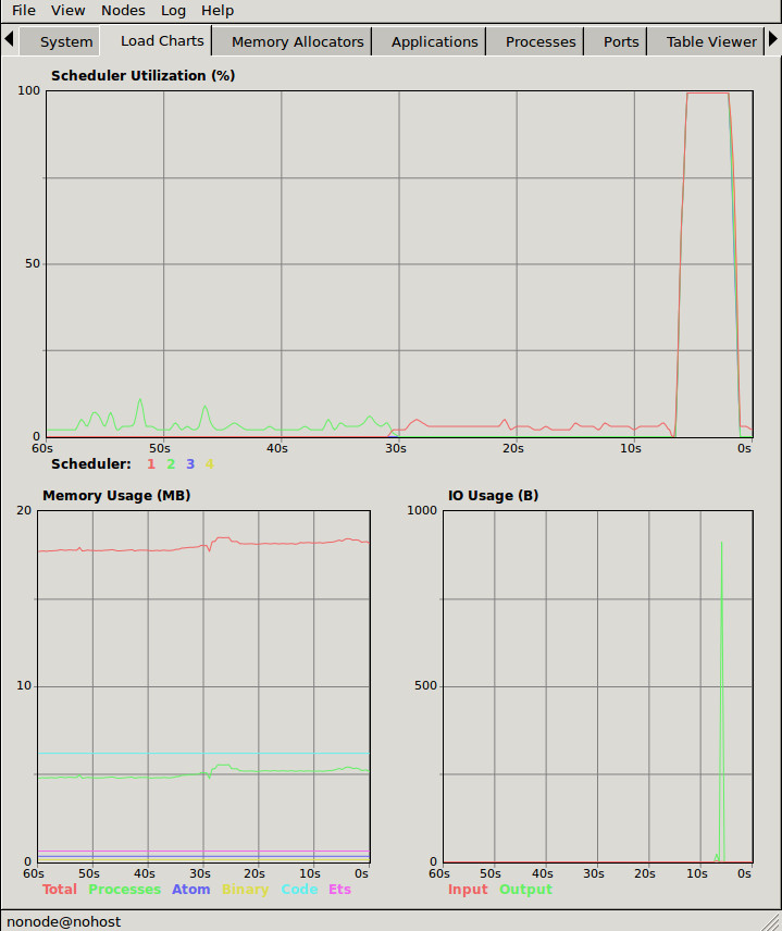
10.2. Preemptive Multitasking in ERTS Cooperating in C
The preemptive multitasking on the Erlang level is achieved by cooperative multitasking on the C level. The Erlang language, the compiler and the virtual machine works together to ensure that the execution of an Erlang process will yield within a limited time and let the next process run. The technique used to measure and limit the allowed execution time is called reduction counting, we will look at all the details of reduction counting soon.
10.3. Reductions
One can describe the scheduling in BEAM as preemptive scheduling on top of cooperative scheduling. A process can only be suspended at certain points of the execution, such as at a receive or a function call. In that way the scheduling is cooperative---a process has to execute code which allows for suspension. The nature of Erlang code makes it almost impossible for a process to run for a long time without doing a function call. There are a few Built In Functions (BIFs) that still can take too long without yielding. Also, if you call C code in a badly implemented Native Implemented Function (NIF) you might block one scheduler for a long time. We will look at how to write well behaved NIFs in Chapter 16.
Since there are no other loop constructs than recursion and
list comprehensions,
there is no way to loop forever without doing a function call.
Each function call is counted as a reduction; when the reduction
limit for the process is reached it is suspended.
|
Version Info
Prior to OTP-20.0, the value of |
|
Reductions
The term reduction comes from the Prolog ancestry of Erlang. In Prolog each execution step is a goal-reduction, where each step reduces a logic problem into its constituent parts, and then tries to solve each part. |
10.3.1. How Many Reductions Will You Get?
When a process is scheduled it will get a number of reductions defined
by CONTEXT_REDS (defined in
erl_vm.h,
currently as 4000). After using up its reductions or when doing a
receive without a matching message in the inbox, the process will be
suspended and a new processes will be scheduled.
If the VM has executed as many reductions as defined by
INPUT_REDUCTIONS (currently 2*CONTEXT_REDS, also defined in
erl_vm.h) or if there is no process ready to run
the scheduler will do system-level activities. That is, basically,
check for IO; we will cover the details soon.
10.3.2. What is a Reduction Really?
It is not completely defined what a reduction is, but at least each function call should be counted as a reduction. Things get a bit more complicated when talking about BIFs and NIFs. A process should not be able to run for "a long time" without using a reduction and yielding. A function written in C can not yield in the middle, it has to make sure it is in a clean state and return. In order to be re-entrant it has to save its internal state somehow before it returns and then set up the state again on re-entry. This can be very costly, especially for a function that sometimes only does little work and sometimes lot. The reason for writing a function in C instead of Erlang is usually to improve performance and to not do unnecessary book keeping work. Since there is no clear definition of what one reduction is, other than a function call on the Erlang level, there is a risk that a function implemented in C takes many more clock cycles per reduction than a normal Erlang function. This can lead to an imbalance in the scheduler, and even starvation.
For example in Erlang versions prior to R16, the BIFs
binary_to_term/1 and term_to_binary/1 were non yielding and only
counted as one reduction. This meant that a process calling these
functions on large terms could starve other processes. This can even
happen in a SMP system because of the way processes are balanced
between schedulers, which we will get to soon.
While a process is running the emulator keeps the number of reductions
left to execute in the (register mapped) variable FCALLS (see
beam_emu.c).
The field reds keep track of the total number of reductions a
process has done up until it was last suspended. By monitoring this
number you can see which processes do the most work.
You can see the total number of reductions for a process (the reds
field) by calling erlang:process_info/2 with the atom reductions
as the second argument. You can also see this number in the process
tab in the observer or with the i/0 command in the Erlang shell.
As noted earlier, each time a process starts the field fcalls is set to
the value of CONTEXT_REDS and for each function call the
process executes fcalls is reduced by 1. When the process is
suspended the field reds is increased by the number of executed
reductions. In some C like code something like:
p→reds += (CONTEXT_REDS - p→fcalls).
Normally a process would do all its allotted reductions and fcalls
would be 0 at this point, but if the process suspends in a receive
waiting for a message it will have some reductions left.
When a process uses up all its reductions it will yield to let another process run, it will go from the process state running to the state runnable, if it yields in a receive it will instead go into the state waiting (for a message). In the next section we will take a look at all the different states a process can be in.
10.4. The Process State (or status)
The field status in the PCB contains the process state. It can be one
of free, runnable, waiting, running, exiting, garbing,
and suspended. When a process exits it is marked as
free---you should never be able to see a process in this state,
it is a short lived state where the process no longer exists as
far as the rest of the system is concerned but there is still
some clean up to be done (freeing memory and other resources).
Each process status represents a state in the Process State Machine. Events such as a timeout or a delivered message triggers transitions along the edges in the state machine. The Process State Machine looks like this:
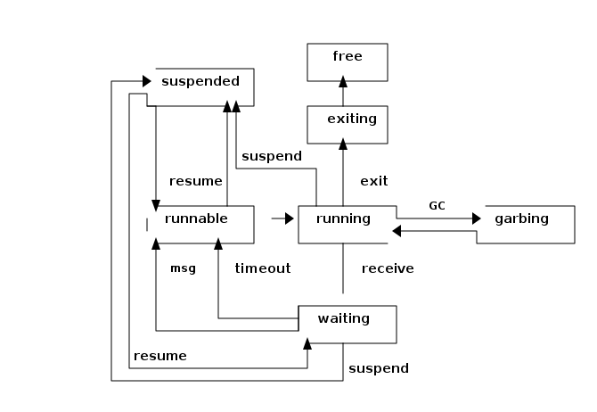
The normal states for a process are runnable, waiting, and running. A running process is currently executing code in one of the schedulers. When a process enters a receive and there is no matching message in the message queue, the process will become waiting until a message arrives or a timeout occurs. If a process uses up all its reductions, it will become runnable and wait for a scheduler to pick it up again. A waiting process receiving a message or a timeout will become runnable.
Whenever a process needs to do garbage collection, it will go into
the garbing
state until the GC is done. While it is doing GC
it saves the old state in the field gcstatus and when it is done
it sets the state back to the old state using gcstatus.
The suspended state is only supposed to be used for debugging
purposes. You can call erlang:suspend_process/2 on another process
to force it into the suspended state. Each time a process calls
suspend_process on another process, the suspend count is increased.
This is recorded in the field rcount.
A call to (erlang:resume_process/1) by the suspending process will
decrease the suspend count. A process in the suspend state will not
leave the suspend state until the suspend count reaches zero.
The field rstatus (resume status) is used to keep track of the
state the process was in before a suspend. If it was running
or runnable it will start up as runnable, and if it was waiting
it will go back to the wait queue. If a suspended waiting process
receives a timeout rstatus is set to runnable so it will resume
as runnable.
To keep track of which process to run next the scheduler keeps the processes in a queue.
10.5. Process Queues
The main job of the scheduler is to keep track of work queues, that is, queues of processes and ports.
There are two process states that the scheduler has to handle, runnable, and waiting. Processes waiting to receive a message are in the waiting state. When a waiting process receives a message the send operations triggers a move of the receiving process into the runnable state. If the receive statement has a timeout the scheduler has to trigger the state transition to runnable when the timeout triggers. We will cover this mechanism later in this chapter.
10.5.1. The Ready Queue
Processes in the runnable state are placed in a FIFO (first in first out) queue handled by the scheduler, called the ready queue. The queue is implemented by a first and a last pointer and by the next pointer in the PCB of each participating process. When a new process is added to the queue the last pointer is followed and the process is added to the end of the queue in an O(1) operation. When a new process is scheduled it is just popped from the head (the first pointer) of the queue.
 The Ready Queue

 First: -->  P5       +---> P3       +-+-> P17
             next: ---+     next: ---+ |  next: NULL
                                       |
 Last: --------------------------------+
In a SMP system, where you have several scheduler threads, there is one queue per scheduler.
 Scheduler 1       Scheduler 2      Scheduler 3      Scheduler 4

 Ready: P5         Ready: P1        Ready: P7        Ready: P9
        P3                P4               P12
        P17                                P10
The reality is slightly more complicated since Erlang processes have priorities. Each scheduler actually has three queues. One queue for max priority tasks, one for high priority tasks and one queue containing both normal and low priority tasks.
 Scheduler 1       Scheduler 2      Scheduler 3      Scheduler 4

 Max:    P5        Max:             Max:             Max:
 High:             High:  P1        High:            High:
 Normal: P3        Ready: P4        Ready: P7        Ready: P9
         P17                               P12
                                           P10
If there are any processes in the max queue the scheduler will pick these processes for execution. If there are no processes in the max queue but there are processes in the high priority queue the scheduler will pick those processes. Only if there are no processes in the max and the high priority queues will the scheduler pick the first process from the normal and low queue.
When a normal process is inserted into the queue it gets a schedule count of 1 and a low priority process gets a schedule count of 8. When a process is picked from the front of the queue its schedule count is reduced by one, if the count reaches zero the process is scheduled, otherwise it is inserted at the end of the queue. This means that low priority processes will go through the queue seven times before they are scheduled.
10.5.2. Waiting, Timeouts and the Timing Wheel
A process trying to do a receive on an empty mailbox or on a mailbox with no matching messages will yield and go into the waiting state.
When a message is delivered to an inbox the sending process will check whether the receiver is sleeping in the waiting state, and in that case it will wake the process, change its state to runnable, and put it at the end of the appropriate ready queue.
If the receive statement has a timeout clause a timer will be
created for the process which will trigger after the specified timeout
time. The only guarantee the runtime system gives on a timeout is that
it will not trigger before the set time. It might be some time after
the intended time before the process is scheduled and gets to execute.
Timers are handled in the VM by a timing wheel. That is, an array of time slots which wraps around. Prior to Erlang 18 the timing wheel was a global resource and there could be some contention for the write lock if you had many processes inserting timers into the wheel. Make sure you are using a later version of Erlang if you use many timers.
The default size (TIW_SIZE) of the timing wheel is 65536 slots (or
8192 slots if you have built the system for a small memory
footprint). The current time is indicated by an index into the array
(tiw_pos). When a timer is inserted into the wheel with a timeout of
T the timer is inserted into the slot at (tiw_pos+T)%TIW_SIZE.
   0 1                                      65535
  +-+-+- ... +-+-+-+-+-+-+-+-+-+-+-+ ... +-+-----+
  | | |      | | | | | | |t| | | | |     | |     |
  +-+-+- ... +-+-+-+-+-+-+-+-+-+-+-+ ... +-+-----+
              ^           ^                       ^
              |           |                       |
           tiw_pos     tiw_pos+T               TIW_SIZE
The timer stored in the timing wheel is a pointer to an ErlTimer
struct. See erl_time.h. If several timers are
inserted into the same slot they are linked together in a linked list
by the prev and next fields. The count field is set to
T/TIW_SIZE
/*
** Timer entry:
*/
typedef struct erl_timer {
    struct erl_timer* next;	/* next entry tiw slot or chain */
    struct erl_timer* prev;	/* prev entry tiw slot or chain */
    Uint slot;			/* slot in timer wheel */
    Uint count;			/* number of loops remaining */
    int    active;		/* 1=activated, 0=deactivated */
    /* called when timeout */
    void (*timeout)(void*);
    /* called when cancel (may be NULL) */
    void (*cancel)(void*);
    void* arg;        /* argument to timeout/cancel procs */
} ErlTimer;
10.6. Ports
A port is an Erlang abstraction for a communication point with the world outside of the Erlang VM. Communications with sockets, pipes, and file IO are all done through ports on the Erlang side.
A port, like a process, is created on the same scheduler as the creating process. Also like processes ports use reductions to decide when to yield, and they also get to run for 4000 reductions. But since ports don’t run Erlang code there are no Erlang function calls to count as reductions, instead each port task is counted as a number of reductions. Currently a task uses a little more than 200 reductions per task, and a number of reductions relative to one thousands of the size of transmitted data.
A port task is one operation on a port, like opening, closing, sending a number of bytes or receiving data. In order to execute a port task the executing thread takes a lock on the port.
Port tasks are scheduled and executed in each iteration in the scheduler loop (see below) before a new process is selected for execution.
10.7. The Scheduler Loop
Conceptually you can look at the scheduler as the driver of program
execution in the Erlang VM. In reality, that is, the way the C code
is structured, it is the emulator (process_main in beam_emu.c) that
drives the execution and it calls the scheduler as a subroutine to find
the next process to execute.
Still, we will pretend that it is the other way around, since it makes a nice conceptual model for the scheduler loop. That is, we see it as the scheduler picking a process to execute and then handing over the execution to the emulator.
Looking at it that way, the scheduler loop looks like this:
-
Update reduction counters.
Each process is allotted a number of reductions (small units of execution). When the reduction count is exceeded, the process is preempted and another is scheduled.
-
Check timers
Timers (e.g.,
receive … after) are checked via a timing wheel. If a timeout has expired, the associated process is moved to the ready queue. -
If needed check balance
The system occasionally checks if some scheduler threads are overloaded. If so, load balancing decisions are made.
-
If needed migrate processes and ports
Processes and ports may be moved between scheduler threads to rebalance CPU load in multicore environments.
-
Do auxiliary scheduler work
This includes handling dirty NIFs, process exits, tracing hooks, and other deferred runtime maintenance tasks.
-
If needed check IO and update time
Polls file descriptors or ports for I/O readiness and may update system time or wall clocks.
-
While needed pick a port task to execute
Tasks such as TCP reads or writes, or invoking driver callbacks, are performed here before scheduling a process.
-
Pick a process to execute
A runnable process is selected from the run queue, considering priority and fairness, and handed to the emulator for execution.
10.8. Load Balancing
The current strategy of the load balancer is to use as few schedulers as possible without overloading any CPU. The idea is that you will get better performance through better memory locality when processes share the same CPU.
One thing to note though is that the load balancing done in the scheduler is between scheduler threads and not necessarily between CPUs or cores. When you start the runtime system you can specify how schedulers should be allocated to cores. The default behaviour is that it is up to the OS to allocated scheduler threads to cores, but you can also choose to bind schedulers to cores.
The load balancer assumes that there is one scheduler running on each core so that moving a process from an overloaded scheduler to an under utilized scheduler will give you more parallel processing power. If you have changed how schedulers are allocated to cores, or if your OS is overloaded or bad at assigning threads to cores, the load balancing might actually work against you.
The load balancer uses two techniques to balance the load, task stealing and migration. Task stealing is used every time a scheduler runs out of work. This technique will result in the work becoming more spread out between schedulers. Migration is more complicated and tries to compact the load to the right number of schedulers.
10.8.1. Task Stealing
If a scheduler run queue is empty when it should pick a new process to schedule the scheduler will try to steal work from another scheduler.
First the scheduler takes a lock on itself to prevent other schedulers to try to steal work from the current scheduler. Then it checks if there are any inactive schedulers that it can steal a task from. If there are no inactive schedulers with stealable tasks then it will look at active schedulers, starting with schedulers having a higher id than itself, trying to find a stealable task.
The task stealing will look at one scheduler at a time and try to steal the highest priority task of that scheduler. Since this is done per scheduler there might actually be higher priority tasks that are stealable on another scheduler which will not be taken.
The task stealing tries to move tasks towards schedulers with lower numbers by trying to steal from schedulers with higher numbers, but since the stealing also will wrap around and steal from schedulers with lower numbers the result is that processes are spread out on all active schedulers.
Task stealing is quite fast and can be done on every iteration of the scheduler loop when a scheduler has run out of tasks.
10.8.2. Migration
To really utilize the schedulers optimally a more elaborate migration strategy is used. The current strategy is to compact the load to as few schedulers as possible, while at the same time spread it out so that no scheduler is overloaded.
This is done by the function check_balance in erl_process.c.
The migration is done by first setting up a migration plan and then letting schedulers execute on that plan until a new plan is set up. Every 2000*CONTEXT_REDS reductions a scheduler calculates a migration path per priority per scheduler by looking at the workload of all schedulers. The migration path can have three different types of values: 1) cleared 2) migrate to scheduler 3) immigrate from scheduler.
When a process becomes ready (for example by receiving a message or triggering a timeout) it will normally be scheduled on the last scheduler it ran on (S1). That is, if the migration path of that scheduler (S1), at that priority, is cleared. If the migration path of the scheduler is set to emigrate (to S2) the process will be handed over to that scheduler if both S1 and S2 have unbalanced run-queues. We will get back to what that means.
When a scheduler (S1) is to pick a new process to execute it checks to see if it has an immigration path from (S2) set. If the two involved schedulers have unbalanced run-queues S1 will steal a process from S2.
The migration path is calculated by comparing the maximum run-queues for each scheduler for a certain priority. Each scheduler will update a counter in each iteration of its scheduler loop keeping track of the maximal queue length. This information is then used to calculate an average (max) queue length (AMQL).
 Max
 Run Q
 Length
    5         o
              o
           o  o
Avg: 2.5 --------------
           o  o     o
    1      o  o     o

scheduler S1 S2 S3 S4
Then the schedulers are sorted on their max queue lengths.
 Max
 Run Q
 Length
    5               o
                    o
                 o  o
Avg: 2.5 --------------
              o  o  o
    1         o  o  o

scheduler S3 S4 S1 S2

           ^        ^
           |        |
          tix      fix
Any scheduler with a longer run queue than average (S1, S2) will be marked for emigration and any scheduler with a shorter max run queue than average (S3, S4) will be targeted for immigration.
This is done by looping over the ordered set of schedulers with two
indices (immigrate from (fix)) and (emigrate to (tix)). In each
iteration of the loop the immigration path of S[tix] is set to S[fix]
and the emigration path of S[fix] is set to S[tix]. Then tix is increased
and fix decreased till they both pass the balance point. If one index
reaches the balance point first it wraps.
In the example:
-
Iteration 1: S2.emigrate_to = S3 and S3.immigrate_from = S2
-
Iteration 2: S1.emigrate_to = S4 and S4.immigrate_from = S1
Then we are done.
In reality things are a bit more complicated since schedulers can be taken offline. The migration planning is only done for online schedulers. Also, as mentioned before, this is done per priority level.
When a process is to be inserted into a ready queue and there is a migration path set from S1 to S2 the scheduler first checks that the run queue of S1 is larger than AMQL and that the run queue of S2 is smaller than the average. This way the migration is only allowed if both queues are still unbalanced.
There are two exceptions though where a migration is forced even when the queues are balanced or even imbalanced in the wrong way. In both these cases a special evacuation flag is set which overrides the balance test.
The evacuation flag is set when a scheduler is taken offline to ensure that no new processes are scheduled on an offline scheduler. The flag is also set when the scheduler detects that no progress is made on some priority. That is, if there for example is a max priority process which always is ready to run so that no normal priority processes ever are scheduled. Then the evacuation flag will be set for the normal priority queue for that scheduler.
11. The Memory Subsystem: Stacks, Heaps and Allocators
Before we dive into the memory subsystem of ERTS, we need to have some basic vocabulary and understanding of the general memory layout of a program in a modern operating system. In this review section I will assume the program is compiled to an ELF executable and running on Linux on something like an IA-32/AMD64 architecture. The layout and terminology is basically the same for all operating systems that ERTS compile on.
A program’s memory layout looks something like this:
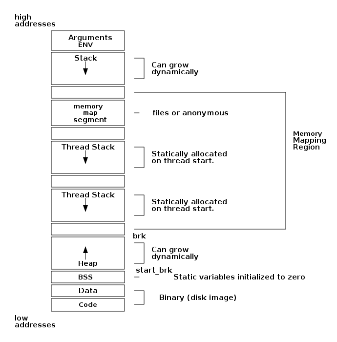
Even though this picture might look daunting it is still a simplification. (For a full understanding of the memory subsystem read a book like "Understanding the Linux Kernel" or "Linux System Programming".) What I want you to take away from this is that there are two types of dynamically allocatable memory: the heap and memory mapped segments. I will try to call this heap the C-heap from now on, to distinguish it from an Erlang process heap. I will call a memory mapped segment for just a segment, and any of the stacks in this picture for the C-stack.
The C-heap is allocated through malloc and a segment is allocated with mmap.
11.1. The Memory Subsystem
Now that we dive into the memory subsystem it will once again be apparent that ERTS is more like an operating system than just a programming language environment. Not only does ERTS provide a garbage collector for Erlang terms on the Erlang process level, but it also provides a plethora of low level memory allocators and memory allocation strategies.
For an overview of memory allocators see the erts_alloc documentation at: http://www.erlang.org/doc/man/erts_alloc.html
All these allocators also come with a number of parameters that can be used to tweak their behavior, and this is probably one of the most important areas from an operational point of view. This is where we can configure the system behavior to fit anything from a small embedded control system (like a Raspberry Pi) to an Internet scale 2TB database server.
There are currently eleven different allocators, six different allocation strategies, and more than 18 other different settings, some of which are taking arbitrary numerical values. This means that there basically is an infinite number of possible configurations. (OK, strictly speaking it is not infinite, since each number is bounded, but there are more configurations than you can shake a stick at.)
In order to be able to use these settings in any meaningful way we will have to understand how these allocators work and how each setting impacts the performance of the allocator.
The erts_alloc manual goes as far as to give the following warning:
Only use these flags if you are absolutely sure what you are doing. Unsuitable settings may cause serious performance degradation and even a system crash at any time during operation.
http://www.erlang.org/doc/man/erts_alloc.html
Making you absolutely sure that you know what you are doing, that is what this chapter is about.
Oh yes, we will also go into details of how the garbage collector works.
11.2. Different Types of Memory Allocators
The Erlang run-time system is trying its best to handle memory in all situations and under all types of loads, but there are always corner cases. In this chapter we will look at the details of how memory is allocated and how the different allocators work. With this knowledge and some tools that we will look at later you should be able to detect and fix problems if your system ends up in one of these corner cases.
For a nice story about the troubles the system might get into and how to analyze and correct the behavior read Fred Hébert’s essay "Troubleshooting Down the Logplex Rabbit Hole".
When we are talking about a memory allocator in this book we have a specific meaning in mind. Each memory allocator manage allocations and deallocations of memory of a certain type. Each allocator is intended for a specific type of data and is often specialized for one size of data.
Each memory allocator implements the allocator interface that can use different algorithms and settings for the actual memory allocation.
The goal with having different allocators is to reduce fragmentation, by grouping allocations of the same size, and to increase performance, by making frequent allocations cheap.
There are two special, fundamental or generic, memory allocator types, sys_alloc and mseg_alloc, and nine specific allocators implemented through the alloc_util framework.
In the following sections we will go though the different allocators, with a little detour into the general framework for allocators (alloc_util).
Each allocator has several names used in the documentation and in the C code. See Table 1 for a short list of all allocators and their names. The C-name is used in the C-code to refer to the allocator. The Type-name is used in erl_alloc.types to bind allocation types to an allocator. The Flag is the letter used for setting parameters of that allocator when starting Erlang.
| Name | Description | C-name | Type-name | Flag |
|---|---|---|---|---|
Basic allocator |
malloc interface |
sys_alloc |
SYSTEM |
Y |
Memory segment allocator |
mmap interface |
mseg_alloc |
- |
M |
Temporary allocator |
Temporary allocations |
temp_alloc |
TEMPORARY |
T |
Heap allocator |
Erlang heap data |
eheap_alloc |
EHEAP |
H |
Binary allocator |
Binary data |
binary_alloc |
BINARY |
B |
ETS allocator |
ETS data |
ets_alloc |
ETS |
E |
Driver allocator |
Driver data |
driver_alloc |
DRIVER |
R |
Short lived allocator |
Short lived memory |
sl_alloc |
SHORT_LIVED |
S |
Long lived allocator |
Long lived memory |
ll_alloc |
LONG_LIVED |
L |
Fixed allocator |
Fixed size data |
fix_alloc |
FIXED_SIZE |
F |
Standard allocator |
For most other data |
std_alloc |
STANDARD |
D |
Literal allocator |
Module constants |
literal_alloc |
LITERAL |
(none) |
11.2.1. The Basic Allocator: sys_alloc
The allocator sys_alloc can not be disabled, and is basically a straight mapping to the underlying OS malloc implementation in libc.
If a specific allocator is disabled then sys_alloc is used instead.
All specific allocators use either sys_alloc or mseg_alloc to allocate memory from the operating system as needed.
When memory is allocated from the OS, sys_alloc can add (pad) a fixed number of kilobytes to the requested number. This can reduce the number of system calls by over allocating memory. The default padding is zero.
When memory is freed, sys_alloc will keep some free memory allocated in the process. The size of this free memory is called the trim threshold, and the default is 128 kilobytes. This also reduces the number of system calls at the cost of a higher memory footprint. This means that if you are running the system with the default settings you can experience that the Beam process does not give memory back to the OS directly as memory is freed up.
Memory areas allocated by sys_alloc are stored in the C-heap of the beam process which will grow as needed through system calls to brk.
11.2.2. The Memory Segment Allocator: mseg_alloc
If the underlying operating system supports mmap a specific memory allocator can use mseg_alloc instead of sys_alloc to allocate memory from the operating system.
Memory areas allocated through mseg_alloc are called segments. When a segment is freed it is not immediately returned to the OS, instead it is kept in a segment cache.
When a new segment is allocated a cached segment is reused if possible, i.e., if it is the same size or larger than the requested size but not too large. The value of absolute max cache bad fit determines the number of kilobytes of extra size which is considered not too large. The default is 4096 kilobytes.
In order not to reuse a 4096 kilobyte segment for really small allocations there is also a relative max cache bad fit value which states that a cached segment may not be used if it is more than that many percent larger. The default value is 20 percent. That is a 12 KB segment may be used when asked for a 10 KB segment.
The number of entries in the cache defaults to 10 but can be set to any value from zero to thirty.
11.2.3. The Memory Allocator Framework: alloc_util
Building on top of the two generic allocators (sys_alloc and mseg_alloc) is a framework called alloc_util which is used to implement specific memory allocators for different types of usage and data.
The framework is implemented in erl_alloc_util.[ch] and the different allocators used by ERTS are defined in erl_alloc.types in the directory "erts/emulator/beam/".
In an SMP system there is usually one allocator of each type per scheduler thread.
The smallest unit of memory that an allocator can work with is called a block. When you call an allocator to allocate a certain amount of memory what you get back is a block. It is also blocks that you give as an argument to the allocator when you want to deallocate memory.
The allocator does not allocate blocks from the operating system directly though. Instead the allocator allocates a carrier from the operating system, either through sys_alloc or through mseg_alloc, which in turn uses malloc or mmap. If sys_alloc is used the carrier is placed on the C-heap, and if mseg_alloc is used the carrier is placed in a segment.
Small blocks are placed in a multiblock carrier. A multiblock carrier can as the name suggests contain many blocks. Larger blocks are placed in a singleblock carrier, which as the name implies contains one block.
What’s considered a small and a large block is determined by the
parameter singleblock carrier threshold (sbct), see the list
of system flags below.
Most allocators also have one "main multiblock carrier" which is never deallocated.
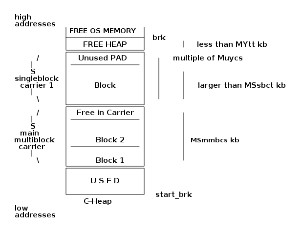
Blocks, Carriers, and Allocation Strategies
When an Erlang process needs memory, it doesn’t directly request it from the
operating system with each allocation. Instead, it interacts with specialized
allocators provided by the alloc_util framework (implemented in
erl_alloc_util.[ch]). These allocators handle requests by distributing memory
from larger contiguous regions known as "carriers."
Carriers are memory regions allocated directly from the operating system. A carrier is allocated either through:
-
sys_alloc(using standard C library functions likemalloc()), placing memory on the process heap, or -
mseg_alloc(usingmmap()), placing memory outside the typical C-heap area.
Carriers are subdivided into smaller memory segments called "blocks." When memory is requested, blocks are allocated from these carriers. There are two primary carrier types:
-
Multiblock Carrier: These hold multiple smaller blocks, suitable for frequent, smaller allocations. By default, allocators typically request multiblock carriers in approximately 8 MB chunks (tunable via system flags), efficiently handling common Erlang memory patterns.
-
Singleblock Carrier: Dedicated to exactly one large block. Allocations exceeding the single block carrier threshold are placed in single-block carriers directly allocated from the OS.
Carrier Threshold (sbct) and Its Impact
The parameter known as singleblock carrier threshold (sbct) determines the
size boundary between what’s considered a "small" and "large" allocation.
Allocations larger than the sbct value use singleblock carriers, while smaller
allocations use multiblock carriers.
By default, the sbct threshold is set so that larger allocations, those significantly bigger than typical Erlang terms—are isolated in single-block carriers. Smaller objects, which constitute most allocations, efficiently share space within multiblock carriers.
This threshold (sbct) is tunable if your application demonstrates unusual allocation patterns. Adjusting it affects how the runtime system balances between fragmentation (caused by large allocations in multiblock carriers) and overhead (due to many single-block carriers).
Why Most Allocations Are Preferably Small (Multiblock Carriers)
Multiblock carriers are favored for their efficiency with typical Erlang workloads—many small, short-lived allocations. Research by the HiPE team has shown most Erlang terms are small (less than eight words), fitting neatly into these multiblock carriers.
A typical ERTS allocator usually maintains:
-
One main multiblock carrier per allocator to handle frequent, small-sized allocations. It rarely releases this carrier, reusing freed blocks internally to reduce fragmentation.
-
Multiple singleblock carriers, each allocated individually for large objects or binaries. Once these blocks are deallocated, the singleblock carriers are returned to the OS immediately.
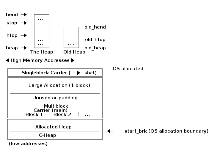
When to Adjust the sbct
Optimizing the singleblock carrier threshold (sbct) parameter is a matter of
understanding your application’s memory allocation patterns. Increasing sbct
directs more allocations into multiblock carriers, improving memory reuse and
reducing fragmentation. This is especially beneficial if your application
frequently allocates moderate-sized data structures, causing fragmentation or
frequent OS-level memory requests.
Reducing sbct, however, forces more allocations into singleblock carriers,
making sense when your application occasionally allocates large memory blocks.
Managing these large allocations separately simplifies their reclamation and
prevents interference with smaller allocations.
If adjusting sbct alone does not resolve frequent minor garbage
collections—often due to numerous short-lived allocations—consider increasing
the process’s initial heap size (min_heap_size) to reduce allocation churn.
In practice, the default sbct setting is suitable for most Erlang
applications. Only fine-tune this parameter if profiling indicates specific
problems with fragmentation, memory overhead, or unusual allocation patterns.
Memory Allocation Strategies
To find a free block of memory in a multi block carrier an
allocation strategy is used. Each type of allocator has
a default allocation strategy, but you can also set the
allocation strategy with the as flag.
The Erlang Run-Time System Application Reference Manual lists the following allocation strategies:
Best fit: Find the smallest block that satisfies the requested block size. (bf)
Address order best fit: Find the smallest block that satisfies the requested block size. If multiple blocks are found, choose the one with the lowest address. (aobf)
Address order first fit: Find the block with the lowest address that satisfies the requested block size. (aoff)
Address order first fit carrier best fit: Find the carrier with the lowest address that can satisfy the requested block size, then find a block within that carrier using the "best fit" strategy. (aoffcbf)
Address order first fit carrier address order best fit: Find the carrier with the lowest address that can satisfy the requested block size, then find a block within that carrier using the "address order best fit" strategy. (aoffcaobf)
Good fit: Try to find the best fit, but settle for the best fit found during a limited search. (gf)
A fit: Do not search for a fit, inspect only one free block to see if it satisfies the request. This strategy is only intended to be used for temporary allocations. (af)
The choice of allocation strategy influences how efficiently free memory is
reused and directly impacts fragmentation and performance. The default strategy
for most allocators is often best fit (bf) or address order best fit
(aobf), which balances memory utilization against allocation speed.
Alternative strategies, such as address order first fit or good fit, can
be configured per allocator (using the +M<S>as <strategy> system flag).
Selecting a different strategy can mitigate memory fragmentation at the expense
of higher CPU overhead during allocation searches.
11.2.4. The Temporary Allocator: temp_alloc
The allocator temp_alloc is used for temporary allocations, that is, very short lived allocations. Memory allocated by temp_alloc may not be allocated over an Erlang process context switch.
You can use temp_alloc as a small scratch or working area while doing some work within a function. Look at it as an extension of the C-stack and free it in the same way. That is, to be on the safe side, free memory allocated by temp_alloc before returning from the function that did the allocation. There is a note in erl_alloc.types saying that you should free a temp_alloc block before the emulator starts executing Erlang code.
Note that no Erlang process running on the same scheduler as the allocator may start executing Erlang code before the block is freed. This means that you can not use a temporary allocation over a BIF or NIF trap (yield).
In a default R16 SMP system there are N+1 temp_alloc allocators where N
is the number of schedulers. The temp_alloc uses the "A fit" (af)
strategy. Since the allocation pattern of the temp_alloc basically is
that of a stack (mostly of size 0 or 1), this strategy works fine.
The temporary allocator is, in R16, used by the following types of data: TMP_HEAP, MSG_ROOTS, ROOTSET, LOADER_TEMP, NC_TMP, TMP, DCTRL_BUF, TMP_DIST_BUF, ESTACK, DB_TMP, DB_MC_STK, DB_MS_CMPL_HEAP, LOGGER_DSBUF, TMP_DSBUF, DDLL_TMP_BUF, TEMP_TERM, SYS_READ_BUF, ENVIRONMENT, CON_VPRINT_BUF.
For an up to date list of allocation types allocated with each
allocator, see erl_alloc.types
(e.g., grep TEMPORARY erts/emulator/beam/erl_alloc.types).
I will not go through each of these different types, but in general as you can guess by their names, they are temporary buffers or work stacks.
11.2.5. The Heap Allocator: eheap_alloc
The heap allocator manages memory blocks for a process’s private data: Erlang
terms stored on the process heap (new and old generations), plus related
structures like heap fragments and beam registers. Almost every Erlang term a
process creates ends up in memory obtained through eheap_alloc.
By default, each scheduler has one eheap_alloc instance, so memory for processes
running on that scheduler remains mostly local, reducing contention. The
allocator’s frequent tasks include:
-
Process Heap: Each Erlang process has its own heap where it stores data such as tuples, lists, maps, integers, and any small binaries (⇐ 64 bytes).
-
Heap Fragments: If a process briefly needs more memory but cannot immediately GC (e.g., constructing a large message), the VM may allocate a “heap fragment” from eheap_alloc. On the next garbage collection, these fragments are merged or freed.
-
Register Arrays: Some runtime-implementation details (e.g., the “beam_registers” data structure) also use eheap_alloc. As an Erlang developer, you typically optimize around eheap_alloc usage by controlling process heap sizes or by understanding when your processes generate large, short-lived data. Good practice includes carefully sizing process heaps if they frequently handle big data, rather than allowing many minor GCs.
11.2.6. The Binary Allocator: binary_alloc
The binary allocator handles memory for (yes, you guessed it) binaries.
Specifically, it manages binaries larger than 64 bytes (called refc binaries),
storing them off-heap and using reference counting to track their usage. Each
process heap holds just a small wrapper (a ProcBin) pointing to the actual
binary.
These binaries vary widely, from modestly sized binaries (hundreds of bytes) up to massive binaries measured in megabytes (such as entire file contents or external data from networks).
The allocator has a few interesting characteristics:
-
Best-Fit Strategy: It chooses the smallest suitable free block to store a new binary, which reduces fragmentation, think of it as a meticulous Tetris player fitting binaries neatly into memory.
-
Reference Counting: Off-heap binaries stick around until the very last process stops referencing them. If just one forgetful process clings to a huge binary, it stays alive, sometimes annoyingly longer than you’d prefer.
-
Sub-Binaries (Slices): When you match binaries like
<<X:32, Rest/binary>>, the smaller binary (Rest) still references the original larger binary, avoiding copying is great, until you realize you’ve accidentally kept a giant binary alive just to reference a tiny bit. In these cases, callingbinary:copy/1is your friend.
If memory mysteriously grows, check for large binaries hanging around due to
references lingering in processes. Occasionally, you might need to gently remind
the garbage collector (via erlang:garbage_collect/1) or let processes
hibernate to reclaim the memory faster.
11.2.7. The ETS Allocator: ets_alloc
The allocator ets_alloc manages memory for your beloved ETS (Erlang Term
Storage) tables. By default, ETS tables aren’t tied to individual processes,
meaning they hang around even when your processes take their garbage out. Keep
in mind a few key details:
-
Long-Lived Data: Once you place data into an ETS table, it moves out of process heaps and settles into its own cozy allocator. Standard process garbage collection won’t tidy up this space. If you want memory back, you must explicitly remove data or delete the table.
-
Diverse Use Cases: This allocator deals with everything ETS-related—from classic hash tables to fancy
ordered_setstructures and internal metadata. Popular or large tables can easily become memory-hungry beasts, so watch out. -
Short-Lived ETS Data: Sometimes ETS might borrow other allocators temporarily, for quick tasks like matching or intermediate results, but the main data lives in
ets_alloc.
Because ETS tables can grow surprisingly large, occasionally check their
size with functions like ets:info(Tab, memory) or keep an eye on overall
ets_alloc usage through your system metrics.
11.2.8. The Driver Allocator: driver_alloc
The driver allocator handles memory for ports, linked-in drivers, and NIF resources. In simpler terms, if you’re reaching beyond Erlang’s safety net—interacting with I/O drivers, external libraries, or file descriptors—you’ll end up here. Key points to keep in mind:
-
Port & Driver Data: Allocations here include structures for network sockets, open file descriptors, and buffers specific to your linked-in drivers.
-
NIF-Allocated Data: When a NIF reaches out with
enif_alloc, the memory ultimately comes from this allocator. The VM politely waits until you callenif_free, or your NIF object gracefully exits the stage, to reclaim this space. -
Potential For External Leaks: Because NIFs and drivers bypass Erlang’s usual memory-safety rules, a misbehaving driver might unintentionally hold onto memory, creating the digital equivalent of a leaky faucet. Keeping an eye on your
driver_allocusage helps catch these drips.
Though developers rarely manipulate driver_alloc directly, it’s wise to
monitor this allocator in production environments, especially if you
are using NIFs.
11.2.9. The Short-Lived Allocator: sl_alloc
The short-lived allocator (sl_alloc) handles memory for data structures with
lifespans that surpass the blink-and-you-miss-it nature of temporary
allocations, but not by much. Think of it as memory that’s sticking around just
long enough to say hello and have a quick coffee before heading out. Typical
examples include:
-
Intermediate Buffers: Small buffers needed for short operations that linger briefly across scheduling points—but definitely don’t plan on staying overnight.
-
Ephemeral Lists: Temporary runtime structures—such as quick-fire system message buffers or short-lived scheduling metadata—that disappear almost as soon as you notice them.
Erlang/OTP leverages sl_alloc for transient operations like match state
objects, ephemeral I/O buffers, and other fleeting entities. Although these
allocations can outlive truly temporary memory, they’re still expected to depart
swiftly, leaving minimal footprints behind.
If your application is particularly chatty—generating numerous short-lived
allocations (such as frequent small driver calls or brief
computations)—sl_alloc might heat up significantly. Checking usage with tools
like recon_alloc:usage() can tell you whether sl_alloc is overused.
11.2.10. The Long-Lived Allocator: ll_alloc
The long lived allocator handles data intended to stay alive for extended periods, often as long as the Erlang node itself. Typical examples include:
-
Atoms: Once created, atoms persist indefinitely, making them permanent residents of
ll_alloc. -
Loaded Modules and Code: Compiled modules, exported functions, and metadata related to anonymous functions (
funs) are stored here. For instance, when you load a module viacode:load_file(my_module), its metadata lands inll_alloc. -
Scheduler and System Structures: Internal runtime structures—like scheduler run queues (
run_queue), pollset information (pollset), and the process registry (proc_tab)—live here because they’re fundamental to VM operations.
Because objects in ll_alloc tend to stick around, this allocator typically
grows slowly but continuously during a node’s lifetime. If your system
frequently loads and unloads modules, you might see fluctuations. For instance,
repeatedly executing hot-code loading without properly unloading old versions
can gradually inflate memory usage in ll_alloc.
In practice, most systems won’t reclaim much memory from here unless you’re
explicitly unloading modules or performing node restarts. Hence, it’s wise to
occasionally glance at recon_alloc:usage(ll_alloc) to detect unexpected spikes
or fragmentation—especially if your application dynamically manages modules or
extensive long-term data.
11.2.11. The Fixed-Size Allocator: fix_alloc
The fixed allocator, fix_alloc, specializes in allocating fixed-size
objects—typically small C structs whose size never changes (e.g., message
references, driver event data, monitors). Since these objects come in uniform
sizes, the allocator can efficiently handle them.
By default, fix_alloc uses "Address Order Best Fit", returning freed objects neatly into lists of same-sized blocks, effectively minimizing fragmentation. Think of it like perfectly stacking identical LEGO bricks rather than randomly tossing different-sized pieces into a box.
Examples include internal VM structures like ErlMessage, monitor references, and scheduler bookkeeping data.
While developers don’t usually interact directly with fix_alloc, it’s essential at the system level. Efficient allocation here ensures the runtime isn’t bogged down managing tiny, fragmented allocations, helping Erlang keep its reputation for handling concurrency gracefully.
11.2.12. The Standard Allocator: std_alloc
When memory doesn’t neatly fit into Erlang’s specialized allocator buckets, it
finds a home in std_alloc—the runtime’s versatile catch-all allocator. Think
of it as Erlang’s “miscellaneous drawer” for memory.
This allocator handles a diverse mix of allocations. This can include references to ephemeral data that’s ambiguously short- or long-lived, dynamically sized structures, VM subsystem data without clear categorization, or simply memory allocations too unique to neatly classify elsewhere.
Just like the other allocators, you can adjust std_alloc behavior with startup
flags such as +Ms or +Msbct. Usually, you leave it alone, but it’s good to
know it’s tweakable when needed.
In troubleshooting, std_alloc can become a prime suspect for unexplained
memory spikes. Tools like erlang:system_info({allocator, std_alloc}) or
recon_alloc can quickly reveal if it’s hoarding more memory than you
anticipated.
Since std_alloc gathers memory requests that defy neat categorization, it’s
normal for it to accumulate significant usage on busy nodes. If you see this
allocator consistently growing, it’s usually a sign to double-check application
behavior or revisit your assumptions about what’s "normal."
11.2.13. The Literal Allocator: literal_alloc
The literal_alloc stores compile-time constants, often called the literal
pool, in loaded Erlang modules. Think of it as the VM’s "read-only memory
shelf," where Erlang safely stores constants like large static binaries, tuples,
or lists defined at compile time.
Unlike typical allocators, literal_alloc is managed globally rather than per
scheduler, as literals aren’t frequently modified or reclaimed during runtime.
Once loaded, these literals remain until their corresponding module is
explicitly purged or reloaded.
Monitoring literal_alloc is usually uneventful, but frequent dynamic module
updates or loading large literal-heavy modules repeatedly might make it worth a
glance.
11.3. Per-Scheduler Allocator Instances
In modern OTP (since R13B), most memory allocators described above (e.g.,
eheap_alloc, binary_alloc, ets_alloc) have multiple instances to minimize
contention in SMP (Symmetric Multi-Processing) environments. By default, each
scheduler thread maintains its own instance of these allocators, plus one
additional instance shared by driver async threads.
This per-scheduler allocation approach partitions memory management, significantly reducing lock contention and improving scalability on multicore systems. It also implies that memory usage and fragmentation are handled separately for each scheduler, which can affect how you interpret memory statistics or troubleshoot memory-related issues.
When examining allocator metrics (e.g., through recon_alloc or
erlang:system_info), you’ll see statistics aggregated across multiple
allocator instances. Be aware of this when analyzing memory patterns.
11.4. System Flags for Memory
Memory allocator system flags follow this syntax:
+M<S><P> <V>-
<S>is a single uppercase letter identifying the allocator. -
<P>specifies the parameter. -
<V>specifies the value to use.
Allocator identifiers (<S>):
-
B: binary_alloc -
D: std_alloc -
E: ets_alloc -
F: fix_alloc -
H: eheap_alloc -
I: literal_alloc -
L: ll_alloc -
M: mseg_alloc -
R: driver_alloc -
S: sl_alloc -
T: temp_alloc -
Y: sys_alloc -
u: alloc_util (affects all alloc_util-based allocators)
11.5. Commonly Used Flags
Allocation Strategy (as):
Determines how memory blocks are selected within carriers.
-
bf: Best fit -
aobf: Address order best fit -
aoff: Address order first fit -
aoffcbf: Address order first fit carrier best fit -
ageffcbf: Age order first fit carrier best fit -
gf: Good fit -
af: A fit
Example:
+MBas bf(Binary allocator uses best-fit strategy.)
Singleblock Carrier Threshold (sbct):
Defines the threshold in KB above which allocations use singleblock carriers.
Example:
+MBsbct 1024(Binary allocations above 1024 KB use singleblock carriers.)
Multiblock Carrier Settings:
-
Smallest (
smbcs) and Largest (lmbcs) Multiblock Carrier Size: Control minimum/maximum sizes for multiblock carriers (KB). -
Carrier Growth Stages (
mbcgs): Defines carrier size growth between minimum and maximum.
Example:
+MBsmbcs 512 +MBlmbcs 8192(Binary allocator multiblock carriers range from 512 KB to 8 MB.)
Abandon Carrier Utilization Limit (acul):
Percentage threshold below which carriers are abandoned and reused.
Example:
+MBacul 50(Binary carriers with utilization below 50% are marked abandoned.)
Abandon Carrier Free Utilization Limit (acful):
Below this utilization, the VM informs the OS that unused memory can be reclaimed.
Example:
+MDacful 10(std_alloc marks memory as reclaimable by OS if utilization is below 10%.)
Multiple Thread-specific Instances (t):
Controls if allocators use multiple instances (one per scheduler).
Example:
+MHt true(eheap_alloc uses separate allocator instances per scheduler thread.)
Allocation Tagging (atags):
Adds tags to allocations, useful for debugging with instrumentation.
Example:
+MRatags true(Enable tagging for driver_alloc.)
11.6. Special Flags for mseg_alloc
mseg_alloc (Memory Segment Allocator) has specific settings:
-
Super Carrier Size (
scs):` +MMscs 1024` (Creates a 1GB super carrier.) -
Use Large Pages (
lp):` +MMlp on` (Enable large/huge pages support.) -
Super Carrier Only (
sco):` +MMsco true` (Allocations occur only within the super carrier.) -
Maximum Cached Segments (
mcs):` +MMmcs 20` (Stores up to 20 cached segments.)
11.7. Special Flags for sys_alloc
sys_alloc interfaces with the system’s malloc:
-
Trim Threshold (
tt): Releases memory back to the OS when the free heap exceeds threshold.` +MYtt 256` (Set trim threshold to 256 KB.) -
Top Pad (
tp): Extra memory malloc requests from OS to reduce subsequent calls.` +MYtp 512` (malloc requests 512 KB padding.)
11.8. Literal Allocator (literal_alloc)
Stores literals (compile-time constants):
-
Literal Super Carrier Size (
scs):` +MIscs 2048` (Set literal allocator super carrier to 2 GB.)
11.9. Global and Convenience Flags
-
Minimal/Maximal Allocation Setup (
ea):` +Mea min|max|config` (Quick configuration presets for all allocators.) -
Lock Physical Memory (
lpm):` +Mlpm all|no` (Locks VM memory into physical RAM.) -
Dirty Allocator Instances (
dai):` +Mdai max|<number>` (Allocator instances specifically for dirty schedulers.)
11.10. Practical Examples
Reduce fragmentation with address-order best fit across all allocators:
+Muas aobfLimit maximum memory for ETS allocator (e.g., 2 GB):
+MEamax 2097152Enable allocation tagging for debugging across all allocators:
+Muatags true11.11. Recommendations
-
Start with default settings unless issues arise.
-
Monitor allocator usage (
erlang:system_info/1,recon_alloc) before tuning. -
Incrementally test changes in controlled environments.
-
Avoid aggressive tuning without benchmarks and profiling.
|
Most memory allocator flags described above are highly implementation-dependent.
Their behavior, availability, and defaults can change or be removed entirely
without prior notice. Moreover, the runtime ( |
11.12. Process Memory
As we saw in Chapter 3, a process is really just a number of memory areas, in this chapter we will look a bit closer at how the stack, the heap and the mailbox are managed.
The default size of the stack and heap is 233 words. This default
size can be changed globally when starting Erlang through the
+h flag. You can also set the minimum heap size when starting
a process with spawn_opt by setting min_heap_size.
Erlang terms are tagged as we saw in Chapter 4, and when they are stored on the heap they are either cons cells or boxed objects.
11.12.1. Term Sharing
Objects on the heap are passed by references within the context of one process. If you call one function with a tuple as an argument, then only a tagged reference to that tuple is passed to the called function. When you build new terms you will also only use references to sub terms.
For example if you have the string "hello" (which is the same as the
list of integers [104,101,108,108,111]) you would get a memory layout
similar to:

If you then create a tuple with two instances of the list, all that is repeated is
the tagged pointer to the list: 00000000000000000000000010000001. The code
L = [104, 101, 108, 108, 111],
T = {L, L}.
would result in a memory layout as seen below, with T pointing to a boxed object at address 136, where we find an ARITYVAL header saying that this is a tuple of size 2 followed by its two elements, both pointing to the same list L at address 128.

This is nice, since it is cheap to do and uses very little space. But if
you send the tuple to another process or do any other type of IO, or any
operations which results in something called a deep copy, then the
data structure is expanded. So if we send the tuple T to another process
P2 (P2 ! T) then the heap of T2 will get a tuple where the first
element points to one copy of the string and the second element to another
copy, doubling the amount of space used. You can see the result of this
in the section on message passing further below.
If you have nested shared tuples, this duplication upon deep copying will grow exponentially with the level of nesting. You can quickly bring down your Erlang node by expanding a highly shared term, see share.erl in the online appendix for the full code example.
-module(share).

-export([share/2, size/0]).

share(0, Y) -> {Y,Y};
share(N, Y) -> [share(N-1, [N|Y]) || _ <- Y].

size() ->
    T = share:share(5,[a,b,c]),
    {{size, erts_debug:size(T)},
     {flat_size, erts_debug:flat_size(T)}}.


 1> timer:tc(fun() -> share:share(10,[a,b,c]), ok end).
 {1131,ok}

 2> share:share(10,[a,b,c]), ok.
 ok

 3> byte_size(term_to_binary(share:share(10,[a,b,c]))), ok.
 HUGE size (13695500364)
 Abort trap: 6
You can calculate the memory size of a shared term and the size of the
expanded size of the term with the functions erts_debug:size/1 and
erts_debug:flat_size/1.
> share:size().
{{size,19386},{flat_size,94110}}
For most applications this is not a problem, but you should be aware of the problem, which can come up in many situations. A deep copy is used for IO, ETS tables, binary_to_term, and message passing.
Let us look in more detail how message passing works.
11.12.2. Message Passing
When a process P1 sends a message M to another (local) process P2, the process P1 first calculates the flat size of M. Then it allocates a new message buffer of that size by doing a heap_alloc of a heap_frag in the local scheduler context.
Given the code in send.erl (see the online appendix) the state of the system could look like this just before the send in p1/1:

Then P1 starts sending the message M to P2. The code in
erl_message.c first calculates the flat size of M (which in our example is
23 words)[5].
Then (in an SMP system) if it can take a lock on P2 and there is enough
room on the heap of P2 it will copy the message to the heap of P2.
If P2 is running (or exiting) or there isn’t enough space on the heap, then a new heap fragment is allocated (of sizeof ErlHeapFragment - sizeof(Eterm) + 23*sizeof(Eterm)) [6] which after initialization will look like:
erl_heap_fragment:
    ErlHeapFragment* next;	    NULL
    ErlOffHeap off_heap:
      erl_off_heap_header* first;   NULL
      Uint64 overhead;                 0
    unsigned alloc_size;	      23
    unsigned used_size;               23
    Eterm mem[1];		       ?
      ... 22 free words
Then the message is copied into the mem part of the heap fragment, and
the first pointer is updated (note that memory addresses increase
downwards in this picture, to match the struct layout):
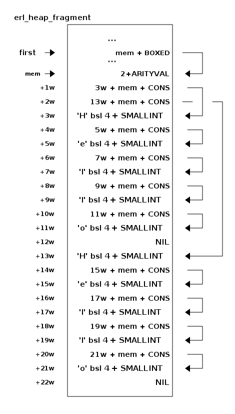
In either case a new mbox (ErlMessage) is allocated, a lock
(ERTS_PROC_LOCK_MSGQ) is taken on the receiver and the message
on the heap or in the new heap fragment is linked into the mbox.
 erl_mesg {
    struct erl_mesg* next = NULL;
    data:  ErlHeapFragment *heap_frag = bp;
    Eterm m[0]            = message;
 } ErlMessage;
Then the mbox is linked into the in message queue (msg_inq) of the
receiver, and the lock is released. Note that msg_inq.last points to
the next field of the last message in the queue. When a new mbox is
linked in, this next pointer is updated to point to the new mbox, and
the last pointer is updated to point to the next field of the new
mbox.
11.12.3. Binaries
As we saw in Chapter 4, there are four types of binaries internally. Three of these types—heap binaries, sub binaries and match contexts—are stored on the local heap and handled by the garbage collector and message passing as any other object, copied as needed.
Reference Counting
The fourth type, large binaries or refc binaries, on the other hand, are partially stored outside of the process heap, and they are reference counted.
The payload of a refc binary is stored in memory allocated by the binary allocator. There is also a small reference to the payload call a ProcBin which is stored on the process heap. This reference is copied by message passing and by the GC, but the payload is untouched. This makes it relatively cheap to send large binaries to other processes since the whole binary doesn’t need to be copied.
All references through a ProcBin to a refc binary increases the reference count of the binary by one. All ProcBin objects on a process heap are linked together in a linked list. After a GC pass this linked list is traversed and the reference count of the binary is decreased with one for each ProcBin that has died. If the reference count of the refc binary reaches zero that binary is deallocated.
Having large binaries reference counted and not copied by send or garbage collection is a big win, but there is one problem with having a mixed environment of garbage collection and reference counting. In a pure reference counted implementation the reference count would be reduced as soon as a reference to the object dies, and when the reference count reaches zero the object is freed. In the ERTS mixed environment a reference to a reference-counted object does not die until a garbage collection detects that the reference is dead.
This means that binaries, which have a tendency to be large or even huge, can hang around for a long time after all references to the binary are dead. Note that since binaries are allocated globally, all references from all processes need to be dead, that is all processes that have seen a binary need to do a GC.
Unfortunately it is not always easy, as a developer, to see which processes have seen a binary in the GC sense of the word seen. Imagine for example that you have a load balancer that receives work items and dispatches them to workers.
In this code there is an example of a loop which doesn’t need to do GC. (See the online appendix for a full example.)
loop(Workers, N) ->
  receive
    WorkItem ->
       Worker = lists:nth(N+1, Workers),
       Worker ! WorkItem,
       loop(Workers, (N+1) rem length(Workers))
  end.
This server will just keep on grabbing references to binaries and never free them, eventually using up all system memory.
When one is aware of the problem it is easy to fix, one can either do a garbage_collect on each iteration of loop or one could do it every five seconds or so by adding an after clause to the receive. (after 5000 → garbage_collect(), loop(Workers, N) ).
Sub Binaries and Matching
When you match out a part of a binary you get a sub binary. This sub binary will be a small structure just containing pointers into the real binary. This increases the reference count for the binary but uses very little extra space.
If a match would create a new copy of the matched part of the binary it would cost both space and time. So in most cases just doing a pattern match on a binary and getting a sub binary to work on is what you want.
There are some degenerate cases, imagine for example that you load a huge file like a book into memory and then you match out a small part like a chapter to work on. The problem is then that the whole of the rest of the book is still kept in memory until you are done with processing the chapter. If you do this for many books, perhaps you want to get the introduction of every book in your file system, then you will keep the whole of each book in memory and not just the introductory chapter. This might lead to huge memory usage.
The solution in this case, when you know you only want one small
part of a large binary and you want to have the small part hanging
around for some time, is to use binary:copy/1. This function
is only used for its side effect, which is to actually copy
the sub binary out of the real binary removing the reference to
the larger binary and therefore hopefully letting it be garbage
collected.
There is a pretty thorough explanation of how binary construction and matching is done in the Erlang documentation: http://www.erlang.org/doc/efficiency_guide/binaryhandling.html.
11.13. Other Interesting Memory Areas
11.13.1. The Atom Table.
Atoms in Erlang are unique identifiers represented as integers internally. All atoms are stored in a global structure known as the atom table. The atom table is a fixed-size structure, meaning there’s an upper limit to how many atoms can exist in a running Erlang system (by default, 1,048,576 atoms). While this might sound like a large number, careless usage (especially dynamically creating atoms from external data) can lead to atom exhaustion, which in turn crashes the entire BEAM VM—an event that’s roughly as pleasant as unexpectedly stepping on a LEGO brick in the middle of the night.
Each entry in the atom table contains metadata about an atom, including its string representation (the text of the atom itself), a unique internal identifier used by the runtime system, and additional information like reference counts and details about its usage in modules or functions.
Erlang maintains atoms through three key memory allocator types:
-
atom_text: Contains the string representations of atoms. This area stores the actual text of atoms. -
atom_tab: Stores the atom table itself—a hash table structure for fast lookup. -
atom_entry: Allocates memory for each atom’s metadata (internal representation, usage counts, etc.).
Atoms are never garbage collected. Once an atom is created, it persists until the VM shuts down. This design decision simplifies implementation (and improves lookup performance), but comes with a risk: an uncontrolled atom creation (commonly through dynamic atom generation via something like list_to_atom/1) can lead to exhausting the atom table. Once the atom limit is reached, attempting to create a new atom results in a runtime error, potentially bringing the node down.
Problems often arise when atoms are created carelessly or dynamically, such as when converting user-provided data directly into atoms, parsing large quantities of untrusted external input, or repeatedly generating atoms within loops or recursive functions. These scenarios can lead to rapid atom table growth, potentially exhausting the atom limit and causing severe system issues.
To avoid this:
-
Always validate or allow-list user input before converting to atoms.
-
Use existing atoms wherever possible or, if dynamic identifiers are required, prefer binaries or strings.
-
Monitor the atom table usage regularly using tools like the Observer or built-in functions like:
-
Atom Count (
erlang:system_info(atom_count)): Number of unique atoms currently loaded. -
Atom Memory (
erlang:memory(atom)): Total bytes used by atoms including overhead. -
Atom Used Memory (
erlang:memory(atom_used)): Only the bytes used by the actual atom strings.
-
A simple check from the Erlang shell can give you a quick indication:
1> erlang:system_info(atom_count).
34319
2> erlang:system_info(atom_limit).
1048576
3> erlang:memory(atom).
336049
4> erlang:memory(atom_used).
324520
If you ever reach the atom limit, you have two practical solutions:
Increase the atom table size (though this is generally a short-term band-aid and should not replace good atom hygiene):
erl +t <new_max_atoms>Redesign your application to avoid the unlimited creation of atoms—typically by using binaries, strings, or integer identifiers instead.
Thus, atoms and their management require care—misuse can cause stability problems—but when handled correctly, they remain an extremely efficient way of referencing static, known keys or identifiers throughout your system.
To safely convert strings to atoms without risk of atom exhaustion, Erlang provides the list_to_existing_atom/1 function. This function will only succeed if the atom already exists. If you attempt to create a new atom with this function, it will throw an exception:
1> list_to_existing_atom("Hello").
** exception error: bad argument
in function  list_to_existing_atom/1
called as list_to_existing_atom("Hello")
*** argument 1: not an already existing atom

2> list_to_existing_atom("true").
true
11.13.2. Code
Another significant memory area is the code area, where compiled Erlang modules are loaded. Erlang modules, once compiled, are loaded into this code area of memory, which is shared among all processes running within the Erlang runtime system. The code area is generally static and persistent, as modules remain loaded unless explicitly unloaded or replaced (through hot-code loading).
When you load or reload modules using functions such as l(Module) or code:load_file(Module), the old code is not immediately removed but kept as the "old" version until no processes reference it. Erlang maintains two versions of each module simultaneously. This allows for safe upgrades without disrupting running processes.
Constants defined in the Erlang code—such as numbers, atoms, and binaries—are stored in a constant pool within the module’s code segment. These constants are efficient in terms of memory usage within a single module, as they are stored only once. However, when constants are used outside of their module—such as during message passing or insertion into ETS tables—they are copied onto the receiving process’s heap, potentially increasing overall memory usage significantly.
Monitoring and managing code memory usage is essential, particularly in long-running systems that frequently perform hot-code upgrades. You can inspect loaded modules and their statuses using built-in functions such as code:all_loaded/0, and erlang:memory(code) to monitor the total memory usage by loaded modules and their constants.
1> erlang:memory(code).
6378630
12. Garbage Collection
When a process runs out of space on the stack and heap the process will try to reclaim space by doing a minor garbage collection. The code for this can be found in erl_gc.c.
12.1. Copying Garbage Collection
ERTS uses a generational copying garbage collector. A copying collector means that during garbage collection all live young terms are copied from the old heap to a new heap. Then the old heap is discarded. A generational collector works on the principle that most terms die young, they are temporary terms created, used, and thrown away. Older terms are promoted to the old generation which is collected more seldom, with the rational that once a term has become old it will probably live for a long time.
Conceptually a garbage collection cycle works as follows:
-
First you collect all roots (e.g. the stack).
-
Then for each root, if the root points to a heap allocated object which doesn’t have a forwarding pointer you copy the object to the new heap. For each copied object update the original with a forwarding pointer to the new copy.
-
Now go through the new heap and do the same as for the roots.
12.1.1. Example
We will go through an example to see how this is done in detail. We will go through a minor collection without an old generation, and we will only use the stack as the root set. In reality the process dictionary, trace data and probe data among other things are also included in the rootset.
Let us look at how the call to garbage_collect behaves in the gc_example.
The code will generate a string which is shared by two
elements of a cons and a tuple, the tuple will the be eliminated
resulting in garbage. After the GC there should only be one string on
the heap. That is, first we generate the term
{["Hello","Hello"], "Hello"} (sharing the same string "Hello" in
all instances. Then we just keep the term ["Hello","Hello"] when
triggering a GC.
| We will take the opportunity to go through how you, on a linux system, can use gdb to examine the behavior of ERTS. You can of course use the debugger of your choice. If you already know how to use gdb or if you have no interest in going into the debugger you can just ignore the meta text about how to inspect the system and just look at the diagrams and the explanations of how the GC works. In Section 18.8.1 we will go through how to use gdb to inspect the system in detail. Here we use some of our own helper scripts that unfortunately have been lost to time. |
-module(gc_example).
-export([example/0]).

example() ->
  T = gen_data(),
  S = element(1, T),
  erlang:garbage_collect(),
  S.

gen_data() ->
 S = gen_string($H, $e, $l, $l, $o),
 T = gen_tuple([S,S],S),
 T.

gen_string(A,B,C,D,E) ->
   [A,B,C,D,E].

gen_tuple(A,B) ->
 {A,B}.
After compiling the example I start an erlang shell, test the call and prepare for a new call to the example (without hitting return):
1> gc_example:example().
["Hello","Hello"]
2> spawn(gc_example,example,[]).
Using gdb to inspect the system
Then I use gdb to attach to my erlang node (OS PID: 2955 in this case)
$ gdb /home/happi/otp/lib/erlang/erts-6.0/bin/beam.smp 2955
| Depending on your settings for ptrace_scope you might have to precede the gdb invocation with 'sudo'. |
Then in gdb I set a breakpoint at the start of the main GC function and let the node continue:
(gdb) break garbage_collect_0
(gdb) cont
Continuing.
Now I hit enter in the Erlang shell and execution stops at the breakpoint:
Breakpoint 1, garbage_collect_0 (A__p=0x7f673d085f88, BIF__ARGS=0x7f673da90340) at beam/bif.c:3771
3771	    FLAGS(BIF_P) |= F_NEED_FULLSWEEP;
Inspecting the PCB
Now we can inspect the PCB of the process:
(gdb) p *(Process *) A__p
$1 = {common = {id = 1408749273747, refc = {counter = 1}, tracer_proc = 18446744073709551611, trace_flags = 0, u = {alive = {
        started_interval = 0, reg = 0x0, links = 0x0, monitors = 0x0, ptimer = 0x0}, release = {later = 0, func = 0x0, data = 0x0,
        next = 0x0}}}, htop = 0x7f6737145950, stop = 0x7f6737146000, heap = 0x7f67371458c8, hend = 0x7f6737146010, heap_sz = 233,
  min_heap_size = 233, min_vheap_size = 46422, fp_exception = 0, hipe = {nsp = 0x0, nstack = 0x0, nstend = 0x0, ncallee = 0x7f673d080000,
    closure = 0, nstgraylim = 0x0, nstblacklim = 0x0, ngra = 0x0, ncsp = 0x7f673d0863e8, narity = 0, float_result = 0}, arity = 0,
  arg_reg = 0x7f673d086080, max_arg_reg = 6, def_arg_reg = {393227, 457419, 18446744073709551611, 233, 46422, 2000}, cp = 0x7f673686ac40,
  i = 0x7f673be17748, catches = 0, fcalls = 1994, rcount = 0, schedule_count = 0, reds = 0, group_leader = 893353197987, flags = 0,
  fvalue = 18446744073709551611, freason = 0, ftrace = 18446744073709551611, next = 0x7f673d084cc0, nodes_monitors = 0x0,
  suspend_monitors = 0x0, msg = {first = 0x0, last = 0x7f673d086120, save = 0x7f673d086120, len = 0, mark = 0x0, saved_last = 0x7d0}, u = {
    bif_timers = 0x0, terminate = 0x0}, dictionary = 0x0, seq_trace_clock = 0, seq_trace_lastcnt = 0,
  seq_trace_token = 18446744073709551611, initial = {393227, 457419, 0}, current = 0x7f673be17730, parent = 1133871366675,
  approx_started = 1407857804, high_water = 0x7f67371458c8, old_hend = 0x0, old_htop = 0x0, old_heap = 0x0, gen_gcs = 0,
  max_gen_gcs = 65535, off_heap = {first = 0x0, overhead = 0}, mbuf = 0x0, mbuf_sz = 0, psd = 0x0, bin_vheap_sz = 46422,
  bin_vheap_mature = 0, bin_old_vheap_sz = 46422, bin_old_vheap = 0, sys_task_qs = 0x0, state = {counter = 41002}, msg_inq = {first = 0x0,
    last = 0x7f673d086228, len = 0}, pending_exit = {reason = 0, bp = 0x0}, lock = {flags = {counter = 1}, queue = {0x0, 0x0, 0x0, 0x0},
    refc = {counter = 1}}, scheduler_data = 0x7f673bd6c080, suspendee = 18446744073709551611, pending_suspenders = 0x0, run_queue = {
    counter = 140081362118912}, hipe_smp = {have_receive_locks = 0}}
Wow, that was a lot of information. The interesting part is about the stack and the heap:
hend = 0x7f6737146010,
stop = 0x7f6737146000,
htop = 0x7f6737145950,
heap = 0x7f67371458c8,
Inspecting the stack
By using some helper scripts (now lost in time) we can inspect the stack and the heap in a meaningful way.
(gdb) source gdb_scripts
(gdb) print_p_stack A__p
0x00007f6737146008 [0x00007f6737145929] cons -> 0x00007f6737145928
(gdb) print_p_heap A__p
0x00007f6737145948 [0x00007f6737145909] cons -> 0x00007f6737145908
0x00007f6737145940 [0x00007f6737145929] cons -> 0x00007f6737145928
0x00007f6737145938 [0x0000000000000080] Tuple size 2
0x00007f6737145930 [0x00007f6737145919] cons -> 0x00007f6737145918
0x00007f6737145928 [0x00007f6737145909] cons -> 0x00007f6737145908
0x00007f6737145920 [0xfffffffffffffffb] NIL
0x00007f6737145918 [0x00007f6737145909] cons -> 0x00007f6737145908
0x00007f6737145910 [0x00007f67371458f9] cons -> 0x00007f67371458f8
0x00007f6737145908 [0x000000000000048f] 72
0x00007f6737145900 [0x00007f67371458e9] cons -> 0x00007f67371458e8
0x00007f67371458f8 [0x000000000000065f] 101
0x00007f67371458f0 [0x00007f67371458d9] cons -> 0x00007f67371458d8
0x00007f67371458e8 [0x00000000000006cf] 108
0x00007f67371458e0 [0x00007f67371458c9] cons -> 0x00007f67371458c8
0x00007f67371458d8 [0x00000000000006cf] 108
0x00007f67371458d0 [0xfffffffffffffffb] NIL
0x00007f67371458c8 [0x00000000000006ff] 111
Here we can see the heap of the process after it has allocated the list "Hello" on the heap and the cons containing that list twice, and the tuple containing the cons and the list. The root set, in this case the stack, contains a pointer to the cons containing two copies of the list. The tuple is dead, that is, there are no references to it.
The garbage collection starts by calculating the root set and by
allocating a new heap (to space). By stepping into the GC code in the
debugger you can see how this is done. I will not go through the
details here. After a number of steps the execution will reach the
point where all terms in the root set are copied to the new heap. This
starts around (depending on version) line 1272 with a while loop in
erl_gc.c.
In our case the root is a cons pointing to address 0x00007f95666597f0 containing the letter (integer) 'H'. When a cons cell is moved from the current heap, called from space, to to space the value in the head (or car) is overwritten with a moved cons tag (the value 0).
Inspecting the heap
After the first step where the root set is moved, the from space and the to space looks like this:
from space:
(gdb) print_p_heap p
0x00007f6737145948 [0x00007f6737145909] cons -> 0x00007f6737145908
0x00007f6737145940 [0x00007f6737145929] cons -> 0x00007f6737145928
0x00007f6737145938 [0x0000000000000080] Tuple size 2
0x00007f6737145930 [0x00007f67371445b1] cons -> 0x00007f67371445b0
0x00007f6737145928 [0x0000000000000000] Tuple size 0
0x00007f6737145920 [0xfffffffffffffffb] NIL
0x00007f6737145918 [0x00007f6737145909] cons -> 0x00007f6737145908
0x00007f6737145910 [0x00007f67371458f9] cons -> 0x00007f67371458f8
0x00007f6737145908 [0x000000000000048f] 72
0x00007f6737145900 [0x00007f67371458e9] cons -> 0x00007f67371458e8
0x00007f67371458f8 [0x000000000000065f] 101
0x00007f67371458f0 [0x00007f67371458d9] cons -> 0x00007f67371458d8
0x00007f67371458e8 [0x00000000000006cf] 108
0x00007f67371458e0 [0x00007f67371458c9] cons -> 0x00007f67371458c8
0x00007f67371458d8 [0x00000000000006cf] 108
0x00007f67371458d0 [0xfffffffffffffffb] NIL
0x00007f67371458c8 [0x00000000000006ff] 111
to space:
(gdb) print_heap n_htop-1 n_htop-2
0x00007f67371445b8 [0x00007f6737145919] cons -> 0x00007f6737145918
0x00007f67371445b0 [0x00007f6737145909] cons -> 0x00007f6737145908
In from space the head of the first cons cell has been overwritten with 0 (looks like a tuple of size 0) and the tail has been overwritten with a forwarding pointer pointing to the new cons cell in the to space. In to space we now have the first cons cell with two backward pointers to the head and the tail of the cons in the from space.
Moving the rest of the heap
When the collector is done with the root set the to space contains
backward pointers to all still live terms. At this point the collector
starts sweeping the to space. It uses two pointers n_hp pointing to
the bottom of the unseen heap and n_htop pointing to the top of the heap.
n_htop:
        0x00007f67371445b8 [0x00007f6737145919] cons -> 0x00007f6737145918
n_hp    0x00007f67371445b0 [0x00007f6737145909] cons -> 0x00007f6737145908
The GC will then look at the value pointed to by n_hp, in this case a
cons pointing back to the from space. So it moves that cons to the to
space, incrementing n_htop to make room for the new cons, and
incrementing n_hp to indicate that the first cons is seen.
from space:

0x00007f6737145948 [0x00007f6737145909] cons -> 0x00007f6737145908
0x00007f6737145940 [0x00007f6737145929] cons -> 0x00007f6737145928
0x00007f6737145938 [0x0000000000000080] Tuple size 2
0x00007f6737145930 [0x00007f67371445b1] cons -> 0x00007f67371445b0
0x00007f6737145928 [0x0000000000000000] Tuple size 0
0x00007f6737145920 [0xfffffffffffffffb] NIL
0x00007f6737145918 [0x00007f6737145909] cons -> 0x00007f6737145908
0x00007f6737145910 [0x00007f67371445c1] cons -> 0x00007f67371445c0
0x00007f6737145908 [0x0000000000000000] Tuple size 0
0x00007f6737145900 [0x00007f67371458e9] cons -> 0x00007f67371458e8
0x00007f67371458f8 [0x000000000000065f] 101
0x00007f67371458f0 [0x00007f67371458d9] cons -> 0x00007f67371458d8
0x00007f67371458e8 [0x00000000000006cf] 108
0x00007f67371458e0 [0x00007f67371458c9] cons -> 0x00007f67371458c8
0x00007f67371458d8 [0x00000000000006cf] 108
0x00007f67371458d0 [0xfffffffffffffffb] NIL
0x00007f67371458c8 [0x00000000000006ff] 111

to space:

n_htop:
        0x00007f67371445c8 [0x00007f67371458f9] cons -> 0x00007f67371458f8
        0x00007f67371445c0 [0x000000000000048f] 72
n_hp    0x00007f67371445b8 [0x00007f6737145919] cons -> 0x00007f6737145918
SEEN    0x00007f67371445b0 [0x00007f67371445c1] cons -> 0x00007f67371445c0
The same thing then happens with the second cons.
from space:

0x00007f6737145948 [0x00007f6737145909] cons -> 0x00007f6737145908
0x00007f6737145940 [0x00007f6737145929] cons -> 0x00007f6737145928
0x00007f6737145938 [0x0000000000000080] Tuple size 2
0x00007f6737145930 [0x00007f67371445b1] cons -> 0x00007f67371445b0
0x00007f6737145928 [0x0000000000000000] Tuple size 0
0x00007f6737145920 [0x00007f67371445d1] cons -> 0x00007f67371445d0
0x00007f6737145918 [0x0000000000000000] Tuple size 0
0x00007f6737145910 [0x00007f67371445c1] cons -> 0x00007f67371445c0
0x00007f6737145908 [0x0000000000000000] Tuple size 0
0x00007f6737145900 [0x00007f67371458e9] cons -> 0x00007f67371458e8
0x00007f67371458f8 [0x000000000000065f] 101
0x00007f67371458f0 [0x00007f67371458d9] cons -> 0x00007f67371458d8
0x00007f67371458e8 [0x00000000000006cf] 108
0x00007f67371458e0 [0x00007f67371458c9] cons -> 0x00007f67371458c8
0x00007f67371458d8 [0x00000000000006cf] 108
0x00007f67371458d0 [0xfffffffffffffffb] NIL
0x00007f67371458c8 [0x00000000000006ff] 111

to space:

n_htop:
        0x00007f67371445d8 [0xfffffffffffffffb] NIL
        0x00007f67371445d0 [0x00007f6737145909] cons -> 0x00007f6737145908
        0x00007f67371445c8 [0x00007f67371458f9] cons -> 0x00007f67371458f8
n_hp    0x00007f67371445c0 [0x000000000000048f] 72
SEEN    0x00007f67371445b8 [0x00007f6737145919] cons -> 0x00007f67371445d0
SEEN    0x00007f67371445b0 [0x00007f67371445c1] cons -> 0x00007f67371445c0
The next element in to space is the immediate 72, which is only
stepped over (with n_hp++). Then there is another cons which is moved.
The same thing then happens with the second cons.
from space:

0x00007f6737145948 [0x00007f6737145909] cons -> 0x00007f6737145908
0x00007f6737145940 [0x00007f6737145929] cons -> 0x00007f6737145928
0x00007f6737145938 [0x0000000000000080] Tuple size 2
0x00007f6737145930 [0x00007f67371445b1] cons -> 0x00007f67371445b0
0x00007f6737145928 [0x0000000000000000] Tuple size 0
0x00007f6737145920 [0x00007f67371445d1] cons -> 0x00007f67371445d0
0x00007f6737145918 [0x0000000000000000] Tuple size 0
0x00007f6737145910 [0x00007f67371445c1] cons -> 0x00007f67371445c0
0x00007f6737145908 [0x0000000000000000] Tuple size 0
0x00007f6737145900 [0x00007f67371445e1] cons -> 0x00007f67371445e0
0x00007f67371458f8 [0x0000000000000000] Tuple size 0
0x00007f67371458f0 [0x00007f67371458d9] cons -> 0x00007f67371458d8
0x00007f67371458e8 [0x00000000000006cf] 108
0x00007f67371458e0 [0x00007f67371458c9] cons -> 0x00007f67371458c8
0x00007f67371458d8 [0x00000000000006cf] 108
0x00007f67371458d0 [0xfffffffffffffffb] NIL
0x00007f67371458c8 [0x00000000000006ff] 111

to space:

n_htop:
        0x00007f67371445e8 [0x00007f67371458e9] cons -> 0x00007f67371458e8
        0x00007f67371445e0 [0x000000000000065f] 101
        0x00007f67371445d8 [0xfffffffffffffffb] NIL
n_hp    0x00007f67371445d0 [0x00007f6737145909] cons -> 0x00007f6737145908
SEEN    0x00007f67371445c8 [0x00007f67371458f9] cons -> 0x00007f67371445e0
SEEN    0x00007f67371445c0 [0x000000000000048f] 72
SEEN    0x00007f67371445b8 [0x00007f6737145919] cons -> 0x00007f67371445d0
SEEN    0x00007f67371445b0 [0x00007f67371445c1] cons -> 0x00007f67371445c0
Now we come to a cons that points to a cell that has already been moved.
The GC sees the IS_MOVED_CONS tag at 0x00007f6737145908 and copies the
destination of the moved cell from the tail (*n_hp++ = ptr[1];). This
way sharing is preserved during GC. This step does not affect from space,
but the backward pointer in to space is rewritten.
to space:

n_htop:
        0x00007f67371445e8 [0x00007f67371458e9] cons -> 0x00007f67371458e8
        0x00007f67371445e0 [0x000000000000065f] 101
n_hp    0x00007f67371445d8 [0xfffffffffffffffb] NIL
SEEN    0x00007f67371445d0 [0x00007f67371445c1] cons -> 0x00007f67371445c0
SEEN    0x00007f67371445c8 [0x00007f67371458f9] cons -> 0x00007f67371445e0
SEEN    0x00007f67371445c0 [0x000000000000048f] 72
SEEN    0x00007f67371445b8 [0x00007f6737145919] cons -> 0x00007f67371445d0
SEEN    0x00007f67371445b0 [0x00007f67371445c1] cons -> 0x00007f67371445c0
Then the rest of the list (the string) is moved.
from space:

0x00007f6737145948 [0x00007f6737145909] cons -> 0x00007f6737145908
0x00007f6737145940 [0x00007f6737145929] cons -> 0x00007f6737145928
0x00007f6737145938 [0x0000000000000080] Tuple size 2
0x00007f6737145930 [0x00007f67371445b1] cons -> 0x00007f67371445b0
0x00007f6737145928 [0x0000000000000000] Tuple size 0
0x00007f6737145920 [0x00007f67371445d1] cons -> 0x00007f67371445d0
0x00007f6737145918 [0x0000000000000000] Tuple size 0
0x00007f6737145910 [0x00007f67371445c1] cons -> 0x00007f67371445c0
0x00007f6737145908 [0x0000000000000000] Tuple size 0
0x00007f6737145900 [0x00007f67371445e1] cons -> 0x00007f67371445e0
0x00007f67371458f8 [0x0000000000000000] Tuple size 0
0x00007f67371458f0 [0x00007f67371445f1] cons -> 0x00007f67371445f0
0x00007f67371458e8 [0x0000000000000000] Tuple size 0
0x00007f67371458e0 [0x00007f6737144601] cons -> 0x00007f6737144600
0x00007f67371458d8 [0x0000000000000000] Tuple size 0
0x00007f67371458d0 [0x00007f6737144611] cons -> 0x00007f6737144610
0x00007f67371458c8 [0x0000000000000000] Tuple size 0

to space:

n_htop:
n_hp
SEEN    0x00007f6737144618 [0xfffffffffffffffb] NIL
SEEN    0x00007f6737144610 [0x00000000000006ff] 111
SEEN    0x00007f6737144608 [0x00007f6737144611] cons -> 0x00007f6737144610
SEEN    0x00007f6737144600 [0x00000000000006cf] 108
SEEN    0x00007f67371445f8 [0x00007f6737144601] cons -> 0x00007f6737144600
SEEN    0x00007f67371445f0 [0x00000000000006cf] 108
SEEN    0x00007f67371445e8 [0x00007f67371445f1] cons -> 0x00007f67371445f0
SEEN    0x00007f67371445e0 [0x000000000000065f] 101
SEEN    0x00007f67371445d8 [0xfffffffffffffffb] NIL
SEEN    0x00007f67371445d0 [0x00007f67371445c1] cons -> 0x00007f67371445c0
SEEN    0x00007f67371445c8 [0x00007f67371445e1] cons -> 0x00007f67371445e0
SEEN    0x00007f67371445c0 [0x000000000000048f] 72
SEEN    0x00007f67371445b8 [0x00007f67371445d1] cons -> 0x00007f67371445d0
SEEN    0x00007f67371445b0 [0x00007f67371445c1] cons -> 0x00007f67371445c0
Example Summary
There are some things to note from this example. When terms are created in Erlang they are created bottom up, starting with the elements. The garbage collector works top down, starting with the top level structure and then copying the elements. This means that the direction of the pointers change after the first GC. This has no real implications but it is good to know when looking at actual heaps. You can not assume that structures should be bottom up.
Also note that the GC does a breath first traversal. This means that locality for one term most often is worse after a GC. With the size of modern caches this should not be a problem. You could of course create a pathological example where it becomes a problem, but you can also create a pathological example where a depth first approach would cause problems.
The third thing to note is that sharing is preserved which is really important otherwise we might end up using more space after a GC than before.
Here’s an expanded explanation about generations:
12.2. Generations in Erlang’s Garbage Collection
Erlang’s BEAM virtual machine uses a generational copying garbage collector, a method that efficiently manages memory based on the observation that most objects "die young". Thus, recent allocations are collected frequently, and surviving data gets promoted to an older generation that is less frequently collected.
The PCB (Process Control Block) contains information about the heap, including:
-
high_water: This pointer marks the boundary between old and new objects on the heap. Objects below this line have survived previous collections and are considered "old". Objects above are newly created and more likely to be short-lived.
-
old_heap: Pointer to the heap area designated for "older" objects. Objects are promoted to this area after surviving a minor garbage collection.
-
old_htop: Indicates the current top position in the old heap, signifying where new objects can be placed upon promotion.
-
old_hend: Marks the end boundary of the old heap area. It serves as a reference limit for when the old heap might require additional garbage collection or resizing.
-
gen_gcs: Counts the number of minor generational garbage collections performed on a process.
-
max_gen_gcs: Defines the maximum number of minor collections before the garbage collector performs a full sweep. This threshold ensures that periodically, the whole heap (both old and new) is cleaned up comprehensively.
Additional PCB memory management-related fields include:
-
off_heap: Contains pointers to off-heap structures that the garbage collector must consider during collections. An example of off-heap data would be larger binaries.
-
mbuf and mbuf_sz: These denote heap fragments (memory buffers, or "m-bufs") used primarily when message-passing contention arises. Messages are copied into m-bufs to avoid lock contention or heap space issues.
-
bin_vheap_sz, bin_vheap_mature, bin_old_vheap_sz, and bin_old_vheap: These relate to binary data stored outside the main heap.
-
bin_vheap_sztracks the size of binaries allocated in the process heap. -
bin_vheap_maturedenotes the mature binary virtual heap size, indicating the size of binaries that have survived garbage collections. -
bin_old_vheap_szandbin_old_vheaprefer specifically to older generations of binaries that have been promoted and tracked separately from younger allocations.
-
12.2.1. Visual Representation of Generational Heaps (conceptual)
We can represent the heap and old heap arrangement as follows (in simplified form):
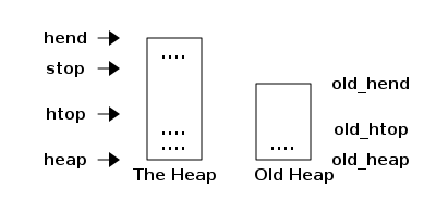
Here, we see a schematic view of two heap areas:
-
The regular heap on the left is where new objects are initially allocated.
-
The old heap on the right stores older, long-lived objects that have survived minor collections and have been promoted to the old generation.
12.3. Practical Implications and Considerations
Frequent minor garbage collections (tracked by gen_gcs) often point to a process that is allocating and discarding short-lived data rapidly. If you see this happening, it’s usually a sign that you can gain performance by optimizing your code paths—particularly by reducing the creation of temporary or intermediate data structures that quickly become garbage. Doing so minimizes garbage collector overhead, leading to more efficient execution and lower CPU usage.
Similarly, observing the high_water pointer moving continuously upward can signal that your process is generating an increasing amount of persistent data. This pattern implies more objects are surviving garbage collection cycles and getting promoted to the old generation, consuming memory over time. Keeping an eye on this helps detect potential memory leaks or inefficiencies in your data lifecycle. Ideally, you want stable heap usage, not a constantly rising tide.
Other important fields such as old_heap, old_htop, and old_hend let you see how much data your process has promoted into the older generation heap, which is collected less frequently. Monitoring these can give insights into whether the process handles long-lived data effectively or if you might be keeping unnecessary references to outdated data.
Similarly, excessive use of memory buffers (mbuf, mbuf_sz) typically signals contention or high throughput in inter-process messaging. If these numbers are growing unusually large, consider rethinking your messaging strategy—perhaps batching messages or restructuring communication patterns. The same principle applies to binary heaps (bin_vheap_sz and bin_vheap_mature). Large binary heaps could indicate a need to reconsider how binaries are handled, ensuring you don’t inadvertently retain large binaries longer than necessary.
12.4. Suggestions for Optimization
Understanding garbage collection in the BEAM VM can provide critical insights into optimizing your application’s performance. Modern hardware has greatly reduced issues related to cache locality, but it’s still important to recognize that the generational garbage collector in Erlang employs a breadth-first copying approach. This method can sometimes degrade data locality, introducing subtle performance nuances that might be noticeable in very performance-sensitive code paths.
In addition, keep an eye on heap fragmentation, particularly the use of memory buffers (m-bufs). If your application heavily relies on message passing, you might experience significant heap fragmentation due to the frequent use of these buffers. Excessive growth of mbuf or mbuf_sz can indicate contention or inefficient message handling. In such scenarios, optimizing message passing strategies by batching messages or rethinking communication patterns can provide significant improvements.
Monitoring garbage collection statistics such as the frequency of minor collections (gen_gcs) and the threshold for major collections (max_gen_gcs) is essential. Regularly reviewing these metrics enables you to detect inefficiencies early, such as excessive temporary data allocation or unintended long-lived data. Identifying these patterns early can help you correct memory inefficiencies and prevent memory leaks or unnecessary garbage collection overhead.
Finally, consider scenarios where your calculation produces large amounts of temporary data. If frequent garbage collections become a bottleneck, proactively setting a larger initial heap size for the process can help. You can achieve this by using Erlang’s spawn_opt with the {min_heap_size, Size} option. This approach reduces GC frequency by ensuring adequate heap space upfront, minimizing performance penalties associated with repeated memory reclamation.
12.5. Stack and Heap Growth
To effectively manage Erlang applications running on the BEAM, you must understand how process memory grows and shrinks. Specifically, processes in Erlang allocate memory dynamically from two primary areas: the stack and the heap.
12.5.1. Stack Growth
The stack holds function calls, return addresses, local variables, and intermediate data needed during computation. When a function call occurs, a new stack frame is created to store parameters, return addresses, and local variables. As your code makes deeper recursive calls, the stack naturally grows, expanding downward toward the heap area. Conversely, as functions complete, the stack shrinks by discarding frames that are no longer needed. The stack grows downward (towards lower memory addresses).
Stack overflow occurs if your function calls become too deeply nested or you use recursion incorrectly. A carefully designed Erlang application should avoid excessively deep recursion or should implement tail-call optimized recursion to prevent unnecessary stack growth.
12.5.2. Heap Growth
The heap, on the other hand, stores Erlang terms like tuples, lists, maps, binaries, and other dynamically allocated structures. Unlike the stack, the heap grows upward (towards higher memory addresses). New data allocated by the process ends up at the top of the heap (htop), continuously moving upward. When the heap runs out of space, a garbage collection is triggered, reclaiming memory from unused terms.
Garbage collection compacts live terms by copying them to a new area, reducing fragmentation. After GC, the heap size might shrink (due to reclaimed memory), remain constant, or grow if insufficient memory is reclaimed to satisfy the process’s needs.
12.5.3. Interaction Between Stack and Heap
In Erlang, the stack and heap are conceptually separate, yet physically co-located within the same contiguous memory block allocated for the process. They grow towards each other:
-
Stack: grows downward (lower addresses).
-
Heap: grows upward (towards higher addresses).
A process runs out of memory if the stack and heap collide—this triggers garbage collection, attempting to reclaim heap space. If insufficient space can be reclaimed, BEAM allocates a larger memory area for the process.
12.5.4. Practical Optimization Advice
Keep an eye on stack depth and heap size during profiling (observer or etop can help with this). You might see excessive heap growth if temporary terms accumulate or if unnecessary copies occur. Also, monitor stack usage for deeply recursive or heavily nested calls.
When your calculation requires a large amount of temporary heap space, consider pre-allocating a larger heap.
Understanding this dynamic stack and heap interaction gives you precise control over your application’s memory behavior, allowing you to write more performant, efficient, and stable Erlang code.
12.6. Key Memory Characteristics and Optimization Opportunities
To deepen your understanding and enhance your approach to memory management and garbage collection (GC) in Erlang and the BEAM, consider the following characteristics and insights from prior research:
12.6.1. No Cycles: Reference Counting or Copying?
In Erlang, terms are immutable, which naturally eliminates the possibility of creating cyclic references in memory. Because of this immutability, Erlang could theoretically use simpler garbage collection strategies such as reference counting. But reference counting comes with its overhead, particularly around frequent updates and multi-threaded contention. Instead, Erlang relies on a copying collector, partly because Erlang terms are usually small, and copying collectors offer better cache locality and minimal fragmentation.
Typical Term Sizes and Distribution
According to research by the HiPE (High-Performance Erlang) team, Erlang terms are typically small and predominantly consist of simple structures. Their measurements found the following approximate term distribution in typical Erlang applications:
-
Approximately 75% of all allocated terms are simple cons cells.
-
About 24% are non-cons terms but smaller than eight words in size.
-
Only around 1% are terms that are equal to or larger than 8 words.
Given these observations, the generational copying garbage collection strategy suits Erlang’s workload particularly well. The majority of terms (around 99%) are short-lived or small, meaning they can be efficiently copied and managed with minimal overhead.
Less Fragmentation, Better Locality with Copying GC
Due to the compact nature of most Erlang terms, a copying garbage collector excels in preserving memory locality and reducing heap fragmentation. With small terms frequently being copied to new heap areas, the garbage collector maintains contiguous memory blocks, enhancing CPU cache locality. In practice, this means improved performance due to fewer cache misses and more predictable memory access patterns.
Implications for Application Optimization
Given these characteristics, the copying garbage collector provides clear advantages:
-
Minimal Fragmentation: Because memory is compacted during each garbage collection, there is very little heap fragmentation. This keeps memory utilization efficient.
-
Improved Locality: Copying live terms to new memory locations in one continuous memory area improves cache locality, enhancing execution speed on modern CPUs.
However, there are trade-offs associated with the copying approach:
-
Copy Overhead: Constantly copying terms around can introduce overhead for larger data structures or long-lived terms, although typically negligible for Erlang’s use case.
-
Potential Impact on Large Terms: While uncommon, large terms (over 8 words, representing roughly 1% of data) might incur performance penalties during copying. Such terms might be optimized by explicit binary or off-heap allocations.
Why Not Reference Counting?
At first glance, Erlang’s lack of cyclic structures suggests a reference-counting strategy could be used. But reference counting incurs overhead every time a term reference changes and does not inherently solve fragmentation issues. Given Erlang’s use case—frequent allocation of small terms—copying collection still outperforms reference counting.
12.6.2. Practical Takeaway
Understanding that Erlang’s data profile fits naturally with generational copying GC clarifies why BEAM employs this method. It emphasizes a strategy for optimization that involves:
-
Minimizing unnecessary allocations and ephemeral data.
-
Avoiding large or complex data structures when possible, or moving large data off the main heap.
-
Setting heap sizes carefully for processes that generate large temporary data.
By aligning your memory management practices with Erlang’s garbage collection strategy, you can optimize your applications for better performance and resource utilization.
13. IO, Ports and Networking
Within Erlang, all communication is done by asynchronous signaling. The communication between an Erlang node and the outside world is done through a port. A port is an interface between Erlang processes and an external resource. In early versions of Erlang a port behaved very much in the same way as a process and you communicated by sending and receiving signals. You can still communicate with ports this way but there are also a number of BIFs to communicate directly with a port.
In this chapter we will look at how ports are used as a common interface for all IO, how ports communicate with the outside world and how Erlang processes communicate with ports. But first we will look at how standard IO works on a higher level.
13.1. Standard IO
Understanding standard I/O in Erlang helps with debugging and interaction with external programs. This section will cover the I/O protocol, group leaders, how to use 'erlang:display', 'io:format', and methods to redirect standard I/O.
13.1.1. I/O Protocol
Erlang’s I/O protocol handles communication between processes and I/O devices. The protocol defines how data is sent to and received from devices like the terminal, files, or external programs. The protocol includes commands for reading, writing, formatting, and handling I/O control operations. These commands are performed asynchronously, maintaining the concurrency model of Erlang. For more detailed information, refer to the official documentation at erlang.org:io_protocol.
The I/O protocol is used to communicate with the group leader, which is responsible for handling I/O requests. The group leader is the process that receives I/O requests from other processes and forwards them to the I/O server. The I/O server is responsible for executing the requests and sending the responses back to the group leader, which then forwards them to the requesting process.
We will discuss group leaders later, but lets look at the actual I/O protocol first. The protocol has the following messages:
Basic Messages
-
{io_request, From, ReplyAs, Request}:-
From:pid()of the client process. -
ReplyAs: Identifier for matching the reply to the request. -
Request: The I/O request.
-
-
{io_reply, ReplyAs, Reply}:-
ReplyAs: Identifier matching the original request. -
Reply: The response to the I/O request.
-
Output Requests
-
{put_chars, Encoding, Characters}:-
Encoding:unicodeorlatin1. -
Characters: Data to be written.
-
-
{put_chars, Encoding, Module, Function, Args}:-
Module, Function, Args: Function to produce the data.
-
Input Requests
-
{get_until, Encoding, Prompt, Module, Function, ExtraArgs}:-
Encoding:unicodeorlatin1. -
Prompt: Data to be output as a prompt. -
Module, Function, ExtraArgs: Function to determine when enough data is read.
-
-
{get_chars, Encoding, Prompt, N}:-
Encoding:unicodeorlatin1. -
Prompt: Data to be output as a prompt. -
N: Number of characters to be read.
-
-
{get_line, Encoding, Prompt}:-
Encoding:unicodeorlatin1. -
Prompt: Data to be output as a prompt.
-
Server Modes
-
{setopts, Opts}:-
Opts: List of options for the I/O server.
-
-
getopts:-
Requests the current options from the I/O server.
-
Multi-Request and Optional Messages
-
{requests, Requests}:-
Requests: List of validio_requesttuples to be executed sequentially.
-
-
{get_geometry, Geometry}:-
Geometry: Requests the number of rows or columns (optional).
-
Unimplemented Request Handling
If an I/O server encounters an unrecognized request, it should respond with:
{error, request}.
Example of a Custom I/O Server
Here’s a simplified example of an I/O server that stores data in memory:
-module(custom_io_server).
-export([start_link/0, stop/1, init/0, loop/1, handle_request/2]).

-record(state, {buffer = <<>>, pos = 0}).

start_link() ->
    {ok, spawn_link(?MODULE, init, [])}.

init() ->
    ?MODULE:loop(#state{}).

stop(Pid) ->
    Pid ! {io_request, self(), Pid, stop},
    receive
        {io_reply, _, {ok, State}} ->
            {ok, State#state.buffer};
        Other ->
            {error, Other}
    end.

loop(State) ->
    receive
        {io_request, From, ReplyAs, Request} ->
            case handle_request(Request, State) of
                {ok, Reply, NewState} ->
                    From ! {io_reply, ReplyAs, Reply},
                    loop(NewState);
                {stop, Reply, _NewState} ->
                    From ! {io_reply, ReplyAs, Reply},
                    exit(normal);
                {error, Reply, NewState} ->
                    From ! {io_reply, ReplyAs, {error, Reply}},
                    loop(NewState)
            end
    end.

handle_request({put_chars, _Encoding, Chars}, State) ->
    Buffer = State#state.buffer,
    NewBuffer = <<Buffer/binary, Chars/binary>>,
    {ok, ok, State#state{buffer = NewBuffer}};
handle_request({get_chars, _Encoding, _Prompt, N}, State) ->
    Part = binary:part(State#state.buffer, State#state.pos, N),
    {ok, Part, State#state{pos = State#state.pos + N}};
handle_request({get_line, _Encoding, _Prompt}, State) ->
    case binary:split(State#state.buffer, <<$\n>>, [global]) of
        [Line|_Rest] ->
            {ok, <<Line/binary, $\n>>, State};
        _ ->
            {ok, State#state.buffer, State}
    end;
handle_request(getopts, State) ->
    {ok, [], State};
handle_request({setopts, _Opts}, State) ->
    {ok, ok, State};
handle_request(stop, State) ->
    {stop, {ok, State}, State};
handle_request(_Other, State) ->
    {error, {error, request}, State}.
We can now use this memory store as an I/O device for example using the file interface.
-module(file_client).
-export([open/0, close/1, write/2, read/2, read_line/1]).

open() ->
    {ok, Pid} = custom_io_server:start_link(),
    {ok, Pid}.

close(Device) ->
    custom_io_server:stop(Device).

write(Device, Data) ->
    file:write(Device, Data).

read(Device, Length) ->
    file:read(Device, Length).

read_line(Device) ->
    file:read_line(Device).
Now we can use this memory store through the file_client interface:
shell V14.2.1 (press Ctrl+G to abort, type help(). for help)
1> {ok, Pid} = file_client:open().
{ok,<0.219.0>}
2> file_client:write(Pid, "Hello, world!\n").
ok
3> R = file_client:close(Pid).
{ok,<<"Hello, world!\n">>}
4>
13.1.2. Group Leader
Group leaders allow you to redirect I/O to the appropriate endpoint. This property is inherited by child processes, creating a chain. By default, an Erlang node has a group leader called 'user' that manages communication with standard input/output channels. All input and output requests go through this process.
Each shell started in Erlang becomes its own group leader. This means functions run from the shell will send all I/O data to that specific shell process. When switching shells with ^G and selecting a shell (e.g., c <number>), a special shell-handling process directs the I/O traffic to the correct shell.
In distributed systems, slave nodes or remote shells set their group leader to a foreign PID, ensuring I/O data from descendant processes is rerouted correctly.
Each OTP application has an application master process acting as a group leader. This has two main uses:
-
It allows processes to access their application’s environment configuration using
application:get_env(Var). -
During application shutdown, the application master scans and terminates all processes with the same group leader, effectively garbage collecting application processes.
Group leaders are also used to capture I/O during tests by common_test and eunit, and the interactive shell sets the group leader to manage I/O.
Group Leader Functions
-
group_leader() → pid(): Returns the PID of the process’s group leader. -
group_leader(GroupLeader, Pid) → true: Sets the group leader ofPidtoGroupLeader.
The group leader of a process is typically not changed in applications with a supervision tree, as OTP assumes the group leader is the application master.
The 'group_leader/2' function uses the 'group_leader' signal to set the group leader of a process. This signal is sent to the process, which then sets its group leader to the specified PID. The group leader can be any process, but it is typically a shell process or an application master.
Example Usage
1> group_leader().
<0.24.0>

2> self().
<0.42.0>

3> group_leader(self(), <0.43.0>).
true
Understanding group leaders and the difference between the BIF display and the function io:format will help you manage basic I/O in Erlang.
-
erlang:display/1: A BIF that writes directly to the standard output, bypassing the Erlang I/O system. -
io:format/1,2: Sends I/O requests to the group leader. If performed via rpc:call/4, the output goes to the calling process’s standard output.
13.1.3. Redirecting Standard IO at Startup (Detached Mode)
In Erlang, redirecting standard I/O (stdin, stdout, and stderr) at startup, especially when running in detached mode, allows you to control where the input and output are directed. This is particularly useful in production environments where you might want to log output to files or handle input from a different source.
Detached Mode
Detached mode in Erlang can be activated by using the -detached flag. This flag starts the Erlang runtime system as a background process, without a connected console. Here’s how to start an Erlang node in detached mode:
erl -sname mynode -setcookie mycookie -detachedWhen running in detached mode, you need to redirect standard I/O manually, as there is no attached console. This can be done by specifying redirection options for the Erlang runtime.
Redirecting Standard Output and Error
To redirect standard output and standard error to a file, use shell redirection or Erlang’s built-in options. Here’s an example of redirecting stdout and stderr to separate log files:
erl -sname mynode -setcookie mycookie -detached > mynode_stdout.log 2> mynode_stderr.logThis command starts an Erlang node in detached mode and redirects standard output to mynode_stdout.log and standard error to mynode_stderr.log.
Alternatively, you can configure this within an Erlang script or startup configuration:
init() ->
    % Redirect stdout and stderr
    file:redirect(standard_output, "mynode_stdout.log"),
    file:redirect(standard_error, "mynode_stderr.log").
Redirecting Standard Input
Redirecting standard input involves providing an input source when starting the Erlang node. For example, you can use a file as the input source:
erl -sname mynode -setcookie mycookie -detached < input_commands.txt13.1.4. Standard Input and Output Summary
Standard output (stdout) is managed by the group leader and is typically directed to the console or a specified log file. Functions such as io:format/1 and io:put_chars/2 send output to the group leader, which handles writing it to the designated output device or file. Standard error (stderr) is similarly managed by the group leader and can also be redirected to log files or other output destinations. Standard input (stdin) is read by processes from the group leader. In detached mode, input can be redirected from a file or another input source.
You can implement your own I/O server using the I/O protocol and you can use that I/O server as a file descriptor or set it as the group leader of a process and redirect I/O through that server.
13.2. Ports
A port is the process-like interface between Erlang processes and everything that is not Erlang processes. The programmer can to a large extent pretend that everything in the world behaves like an Erlang process and communicate through message passing.
Each port has an owner, more on this later, but all processes that know about the port can send messages to the port. In the figure below we see how a process can communicate with the port and how the port is communicating to the world outside the Erlang node.
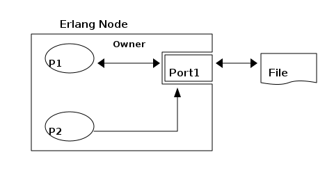
Process P1 has opened a port (Port1) to a file, and is the owner of the port and can receive messages from the port. Process P2 also has a handle to the port and can send messages to the port. The processes and the port reside in an Erlang node. The file lives in the file and operating system on the outside of the Erlang node.
If the port owner dies or is terminated the port is also killed. When a port terminates all external resources should also be cleaned up. This is true for all ports that come with Erlang and if you implement your own port you should make sure it does this cleanup.
13.2.1. Different Types of Ports
There are three different classes of ports: file descriptors, external programs and drivers. A file descriptor port makes it possible for a process to access an already opened file descriptor. A port to an external program invokes the external program as a separate OS process. A driver port requires a driver to be loaded in the Erlang node.
All ports are created by a call to erlang:open_port(PortName,
PortSettings).
A file descriptor port is opened with {fd, In, Out} as the
PortName. This class of ports is used by some internal ERTS servers
like the old shell. They are considered to not be very efficient and
hence seldom used. Also the file descriptors are non-negative integers
representing open file descriptors in the OS. The file descriptor can
not be an erlang I/O server.
An external program port can be used to execute any program in the
native OS of the Erlang node. To open an external program port you
give either the argument {spawn, Command} or {spawn_executable,
FileName} with the name of the external program. This is the easiest
and one of the safest way to interact with code written in other
programming languages. Since the external program is executed in its
own OS process it will not bring down the Erlang node if it
crashes. (It can of course use up all CPU or memory or do a number of
other things to bring down the whole OS, but it is much safer than a
linked in driver or a NIF).
A driver port requires that a driver program has been loaded with
ERTS. Such a port is started with either {spawn, Command} or
{spawn_driver, Command}. Writing your own linked in driver can be an
efficient way to interface for example some C library code that you
would like to use. Note that a linked in driver executes in the same
OS process as the Erlang node and a crash in the driver will bring
down the whole node. Details about how to write an Erlang driver in
general can be found in Chapter 16.
Erlang/OTP comes with a number port drivers implementing the
predefined port types. There are the common drivers available on all
platforms: tcp_inet, udp_inet, sctp_inet, efile, zlib_drv,
ram_file_drv, binary_filer, tty_sl. These drivers are used to
implement, e.g., file handling and sockets in Erlang. On Windows there
is also a driver to access the registry: registry_drv. And on most
platforms there are example drivers to use when implementing your own
driver like: multi_drv and sig_drv.
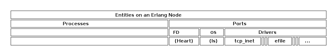
Data sent to and from a port are byte streams. The packet size can be specified in the PortSettings when opening a port. Since R16, ports support truly asynchronous communication, improving efficiency and performance.
Ports can be used to replace standard IO and polling. This is useful when you need to interact with external programs or devices. By opening a port to a file descriptor, you can read and write data to the file. Similarly, you can open a port to an external program and communicate with it using the port interface.
Ports to File Descriptors
File descriptor ports in Erlang provide an interface to interact with already opened file descriptors. Although they are not commonly used due to efficiency concerns, they can provide an easy interface to external resources.
To create a file descriptor port, you use the open_port/2 function with the {fd, In, Out} tuple as the PortName. Here, In and Out are the file descriptors for input and output, respectively.
Bad example:
Port = open_port({fd, 0, 1}, []).This opens a port that reads from the standard input (file descriptor 0) and writes to the standard output (file descriptor 1). Don’t try this example since it will steal the IO from your erlang shell.
You tried it anyway didn’t you? Now you have to restart the shell.
File descriptor ports are implemented using the open_port/2 function, which creates a port object. The port object handles the communication between the Erlang process and the file descriptor.
Internally, when open_port/2 is called with {fd, In, Out}, the Erlang runtime system sets up the necessary communication channels to interact with the specified file descriptors. The port owner process can then send and receive messages to/from the port, which in turn interacts with the file descriptor.
Ports to Spawned OS Processes
To create a port to a spawned OS process, you use the open_port/2 function with the {spawn, Command} or {spawn_executable, FileName} tuple as the PortName. This method allows Erlang processes to interact with external programs by spawning them as separate OS processes.
The primary commands for interacting with a port include:
-
{command, Data}: SendsDatato the external program. -
{control, Operation, Data}: Sends a control command to the external program. -
{exit_status, Status}: Receives the exit status of the external program.
See Chapter 16 for examples of how to spawn an external program as a port. You can also look at the official documentation: erlang.org:c_port.
Ports to Linked-in Drivers
Linked-in drivers in Erlang are created using the open_port/2 function with the {spawn_driver, Command} tuple as the PortName. This method requires the first token of the command to be the name of a loaded driver.
Port = open_port({spawn_driver, "my_driver"}, []).Commands for interacting with a linked-in driver port typically include:
-
{command, Data}: SendsDatato the driver. -
{control, Operation, Data}: Sends a control command to the driver. Example:
Port ! {self(), {command, <<"Hello, Driver!\n">>}}.See Chapter 16 for examples of how to implement and spawn a linked in driver as a port. You can also look at the official documentation: erlang.org:c_portdriver.
13.2.2. Flow Control in Erlang Ports
Ports implement flow control mechanisms to manage backpressure and ensure efficient resource usage. One primary mechanism is the busy port functionality, which prevents a port from being overwhelmed by too many simultaneous operations. When a port is in a busy state, it can signal to the Erlang VM that it cannot handle more data until it processes existing data.
When the port’s internal buffer exceeds a specified high-water mark, the port enters a busy state. In this state, it signals to the VM to stop sending new data until it can process the buffered data.
Processes attempting to send data to a busy port are suspended until the port exits the busy state. This prevents data loss and ensures that the port can handle all incoming data efficiently.
Once the port processes enough data to fall below a specified low-water mark, it exits the busy state. Suspended processes are then allowed to resume sending data.
By scheduling signals to/from the port asynchronously, Erlang ensures that processes sending data can continue executing without being blocked, improving system parallelism and responsiveness.
Now this means that the erlang send operation is not always asynchronous. If the port is busy the send operation will block until the port is not busy anymore. This is a problem if you have a lot of processes sending data to the same port. The solution is to use a port server that can handle the backpressure and make sure that the send operation is always asynchronous.
Let’s do an example based on the official port driver example: erlang.org:c-driver.
Let us use the original complex c function, adding 1 or multiplying by 2.
/* example.c */

int foo(int x)
{
    return x + 1;
}

int bar(int y)
{
    return y * 2;
}
And a slightly modified port driver. We have added an id to each message
and return the id with the result. We also have a function
that simulates a busy port by sleeping for a while and setting
the busy port status if the id of the message is below 14 and the call is to the bar function.
/* Derived from port_driver.c
   https://www.erlang.org/doc/system/c_portdriver.html

*/

#include "erl_driver.h"
#include <stdio.h>
#include <unistd.h> // Include for sleep function

int foo(int x);
int bar(int y);

typedef struct
{
    ErlDrvPort port;
} example_data;

static ErlDrvData bp_drv_start(ErlDrvPort port, char *buff)
{
    example_data *d = (example_data *)driver_alloc(sizeof(example_data));
    d->port = port;
    return (ErlDrvData)d;
}

static void bp_drv_stop(ErlDrvData handle)
{
    driver_free((char *)handle);
}

static void bp_drv_output(ErlDrvData handle, char *buff,
                          ErlDrvSizeT bufflen)
{
    example_data *d = (example_data *)handle;
    char fn = buff[0], arg = buff[1], id = buff[2];
    static char res[2];

    if (fn == 1)
    {
        res[0] = foo(arg);
    }
    else if (fn == 2)
    {
        res[0] = bar(arg);
        if (id > 14)
        {
            // Signal that the port is free
            set_busy_port(d->port, 0);
        }
        else
        {
            // Signal that the port is busy
            // This is not essential for this example
            // However, if multiple processes attempted to use the port
            // in parallel, we would need to signal that the port is busy
            // This would make even the foo function block.
            set_busy_port(d->port, 1);
            // Simulate processing delay
            sleep(1);
            set_busy_port(d->port, 0);
        }
    }
    res[1] = id;
    driver_output(d->port, res, 2);
}

ErlDrvEntry bp_driver_entry = {
    NULL,                           /* F_PTR init, called when driver is loaded */
    bp_drv_start,                   /* L_PTR start, called when port is opened */
    bp_drv_stop,                    /* F_PTR stop, called when port is closed */
    bp_drv_output,                  /* F_PTR output, called when erlang has sent */
    NULL,                           /* F_PTR ready_input, called when input descriptor ready */
    NULL,                           /* F_PTR ready_output, called when output descriptor ready */
    "busy_port_drv",                /* char *driver_name, the argument to open_port */
    NULL,                           /* F_PTR finish, called when unloaded */
    NULL,                           /* void *handle, Reserved by VM */
    NULL,                           /* F_PTR control, port_command callback */
    NULL,                           /* F_PTR timeout, reserved */
    NULL,                           /* F_PTR outputv, reserved */
    NULL,                           /* F_PTR ready_async, only for async drivers */
    NULL,                           /* F_PTR flush, called when port is about
                       to be closed, but there is data in driver
                       queue */
    NULL,                           /* F_PTR call, much like control, sync call
                       to driver */
    NULL,                           /* unused */
    ERL_DRV_EXTENDED_MARKER,        /* int extended marker, Should always be
                       set to indicate driver versioning */
    ERL_DRV_EXTENDED_MAJOR_VERSION, /* int major_version, should always be
                       set to this value */
    ERL_DRV_EXTENDED_MINOR_VERSION, /* int minor_version, should always be
                       set to this value */
    0,                              /* int driver_flags, see documentation */
    NULL,                           /* void *handle2, reserved for VM use */
    NULL,                           /* F_PTR process_exit, called when a
                       monitored process dies */
    NULL                            /* F_PTR stop_select, called to close an
                       event object */
};

DRIVER_INIT(busy_port_drv) /* must match name in driver_entry */
{
    return &bp_driver_entry;
}
Now we can call this function from Erlang synchronously, or send asyncronus messages. In our port handler we have also added some tests that sends 10 messages to the port and then receives the results both synchronously and asynchronously.
%% Derived from https://www.erlang.org/doc/system/c_portdriver.html

-module(busy_port).
-export([start/1, stop/0, init/1]).
-export([foo/1, bar/1, async_foo/1, async_bar/1, async_receive/0]).
-export([test_sync_foo/0,
         test_async_foo/0,
         test_async_bar/0]).

start(SharedLib) ->
    case erl_ddll:load_driver(".", SharedLib) of
	    ok -> ok;
	    {error, already_loaded} -> ok;
	    _ -> exit({error, could_not_load_driver})
    end,
    spawn(?MODULE, init, [SharedLib]).

init(SharedLib) ->
    register(busy_port_example, self()),
    Port = open_port({spawn, SharedLib}, []),
    loop(Port, [], 0).

test_sync_foo() ->
    [foo(N) || N <- lists:seq(1, 10)].

test_async_foo() ->
    [async_receive() || _ <- [async_foo(N) || N <- lists:seq(1, 10)]].

test_async_bar() ->
    [async_receive() || _ <- [async_bar(N) || N <- lists:seq(1, 10)]].


stop() ->
    busy_port_example ! stop.

foo(X) ->
    call_port({foo, X}).
bar(Y) ->
    call_port({bar, Y}).

async_foo(X) ->
    send_message({foo, X}).
async_bar(Y) ->
    send_message({bar, Y}).

async_receive() ->
    receive
        {busy_port_example, Data} ->
            Data
    after 2000 -> timeout
    end.

call_port(Msg) ->
    busy_port_example ! {call, self(), Msg},
    receive
	{busy_port_example, Result} ->
	    Result
    end.

send_message(Message) ->
    busy_port_example ! {send, self(), Message}.


reply(Id, [{Id, From}|Ids], Data) ->
    From ! {busy_port_example, Data},
    Ids;
reply(Id, [Id1|Ids], Data) ->
    [Id1 | reply(Id, Ids, Data)];
reply(_Id, [], Data) -> %% oops, no id found
    io:format("No ID found for data: ~p~n", [Data]),
    [].


loop(Port, Ids, Id) ->
    receive
	{call, Caller, Msg} ->
        io:format("Call: ~p~n", [Msg]),
	    Port ! {self(), {command, encode(Msg, Id)}},
	    receive
		{Port, {data, Data}} ->
            Res = decode_data(Data),
            io:format("Received data: ~w~n", [Res]),
		    Caller ! {busy_port_example, Res}
	    end,
	    loop(Port, Ids, Id);
     {Port, {data, Data}} ->
            {Ref, Res} = decode(Data),
            io:format("Received data: ~w~n", [Res]),
            NewIds = reply(Ref, Ids, Res),
            loop(Port, NewIds, Id);
     {send, From, Message} ->
            T1 = os:system_time(millisecond),
            io:format("Send: ~p~n", [Message]),
            Port ! {self(), {command, encode(Message, Id)}},
            T2 = os:system_time(millisecond),
            if (T2 - T1) > 500 -> io:format("Shouldn't ! be async...~n", []);
               true -> ok
            end,
            loop(Port, [{Id, From} | Ids], Id + 1);
	stop ->
	    Port ! {self(), close},
	    receive
		{Port, closed} ->
		    exit(normal)
	    end;
	{'EXIT', Port, Reason} ->
	    io:format("~p ~n", [Reason]),
	    exit(port_terminated)
    end.

encode({foo, X}, Id) -> [1, X, Id];
encode({bar, X}, Id) -> [2, X, Id].

decode([Int, Id]) -> {Id, Int}.
decode_data([Int,_Id]) -> Int.
Let’s try this in the shell:
1> c(busy_port).
{ok,busy_port}
2> busy_port:start("busy_port_drv").
<0.89.0>
3> busy_port:test_sync_foo().
Call: {foo,1}
Received data: 2
Call: {foo,2}
Received data: 3
Call: {foo,3}
Received data: 4
Call: {foo,4}
Received data: 5
Call: {foo,5}
Received data: 6
Call: {foo,6}
Received data: 7
Call: {foo,7}
Received data: 8
Call: {foo,8}
Received data: 9
Call: {foo,9}
Received data: 10
Call: {foo,10}
Received data: 11
[2,3,4,5,6,7,8,9,10,11]
That worked as expected; we did a synchronous call and immediately got a response. Now let’s try the asynchronous call:
4> busy_port:test_async_foo().
Send: {foo,1}
Send: {foo,2}
Send: {foo,3}
Send: {foo,4}
Send: {foo,5}
Send: {foo,6}
Send: {foo,7}
Send: {foo,8}
Send: {foo,9}
Send: {foo,10}
Received data: 2
Received data: 3
Received data: 4
Received data: 5
Received data: 6
Received data: 7
Received data: 8
Received data: 9
Received data: 10
Received data: 11
[2,3,4,5,6,7,8,9,10,11]That also worked as expected: we sent 10 messages and got the results back in the same order also immediately. Now let’s try the busy port:
5> busy_port:test_async_bar().
Send: {bar,1}
Shouldn't ! be async...
Send: {bar,2}
Shouldn't ! be async...
Send: {bar,3}
Shouldn't ! be async...
Send: {bar,4}
Shouldn't ! be async...
Send: {bar,5}
Shouldn't ! be async...
Send: {bar,6}
Send: {bar,7}
Send: {bar,8}
Send: {bar,9}
Send: {bar,10}
Received data: 2
Received data: 4
Received data: 6
Received data: 8
Received data: 10
Received data: 12
Received data: 14
Received data: 16
Received data: 18
Received data: 20
[timeout,2,4,6,8,10,12,14,16,18]We see that the first 5 messages are not asynchronous, but the last 5 are. This is because the port is busy and the send operation is blocking. The port is busy because the id of the message is below 14 and the call is to the bar function. The port is busy for 5 seconds and then the last 5 messages are sent asynchronously.
13.2.3. Port Scheduling
Erlang ports, similar to processes, execute code (drivers) to handle external communication, such as TCP. Originally, port signals were handled synchronously, causing issues with I/O event parallelism. This was problematic due to heavy lock contention and reduced parallelism potential.
To address these issues, Erlang schedules all port signals, ensuring sequential execution by a single scheduler. This eliminates contention and allows processes to continue executing Erlang code in parallel.
Ports have a task queue managed by a "semi-locked" approach with a public locked queue and a private lock-free queue. Tasks are moved between these queues to avoid lock contention. This system handles I/O signal aborts by marking tasks as aborted using atomic operations, ensuring tasks are safely deallocated without lock contention.
Ports can enter a busy state when overloaded with command signals, suspending new signals until the queue is manageable. This ensures flow control, preventing the port from being overwhelmed before it can process signals.
Signal data preparation occurs before acquiring the port lock, reducing latency. Non-contended signals are executed immediately, maintaining low latency, while contended signals are scheduled for later execution to preserve parallelism.
See Chapter Chapter 10 for details of how the scheduler works and how ports fit into the general scheduling scheme.
13.3. Distributed Erlang
See chapter Chapter 14 for details on the built in distribution layer.
13.4. Sockets, UDP and TCP
Sockets are a fundamental aspect of network communication in Erlang. They allow processes to communicate over a network using protocols such as TCP and UDP. Here, we will explore how to work with sockets, retrieve information about sockets, and tweak socket behavior.
Erlang provides a robust set of functions for creating and managing sockets. The gen_tcp and gen_udp modules facilitate the use of TCP and UDP protocols, respectively. Here is a basic example of opening a TCP socket:
% Open a listening socket on port 1234
{ok, ListenSocket} = gen_tcp:listen(1234, [binary, {packet, 0}, {active, false}, {reuseaddr, true}]),
% Accept a connection
{ok, Socket} = gen_tcp:accept(ListenSocket),
% Send and receive data
ok = gen_tcp:send(Socket, <<"Hello, World!">>),
{ok, Data} = gen_tcp:recv(Socket, 0).For UDP, the process is similar but uses the gen_udp module:
% Open a UDP socket on port 1234
{ok, Socket} = gen_udp:open(1234, [binary, {active, false}]),
% Send and receive data
ok = gen_udp:send(Socket, "localhost", 1234, <<"Hello, World!">>),
receive
{udp, Socket, Host, Port, Data} -> io:format("Received: ~p~n", [Data])
end.Erlang provides several functions to retrieve information about sockets. For instance, you can use inet:getopts/2 and inet:setopts/2 to get and set options on sockets. Here’s an example:
% Get options on a socket
{ok, Options} = inet:getopts(Socket, [recbuf, sndbuf, nodelay]),
% Set options on a socket
ok = inet:setopts(Socket, [{recbuf, 4096}, {sndbuf, 4096}, {nodelay, true}]).Additionally, you can use inet:peername/1 and inet:sockname/1 to get the remote and local addresses of a socket:
% Get the remote address of a connected socket
{ok, {Address, Port}} = inet:peername(Socket),
% Get the local address of a socket
{ok, {LocalAddress, LocalPort}} = inet:sockname(Socket).To optimize socket performance and behavior, you can tweak various socket options. Commonly adjusted options include buffer sizes, timeouts, and packet sizes. Here’s how you can tweak some of these options:
% Set socket buffer sizes
ok = inet:setopts(Socket, [{recbuf, 8192}, {sndbuf, 8192}]),
% Set a timeout for receiving data
ok = inet:setopts(Socket, [{recv_timeout, 5000}]),
% Set packet size for a TCP socket
ok = inet:setopts(Socket, [{packet, 4}]).14. Distribution
Erlang is designed to support distributed computing. This chapter will explore the key aspects of distribution in Erlang, including nodes, connections, and message passing.
14.1. Nodes and Connections
In Erlang, a node is an instance of the Erlang runtime system. According to the specification it is actually a named running instance of ERTS, since only named instances can communicate through the Erlang distributions.
In this book we will often, a bit erroneously, also refer to non distributed, unnamed instances as nodes. They can still communicate with other subsystems for example through http or directly through TCP.
Each real node has a unique name, which is typically composed of an atom followed by an '@' symbol and the hostname. For example, node1@localhost.
The name of a node can be either a short name or a long name. A short name is composed of an atom and does not include the hostname, like node1. Short names are used when all nodes are running on the same host. A long name, on the other hand, includes both the atom and the hostname, like node1@localhost. Long names are used when nodes are distributed across different hosts. It’s important to note that nodes using short names can only communicate with other nodes using short names, and nodes using long names can only communicate with nodes using long names. Therefore, it’s crucial to be consistent with the naming scheme across all nodes in a distributed system.
Nodes can establish connections with each other using the net_kernel:connect_node/1 function.
The name of a node is composed of two parts: a name (which is an atom), and a hostname. The format is name@hostname.
If we start a node without a name we can not connect to another node:
happi@gdc12:~$ iex
Erlang/OTP 24 [erts-12.0.4] [source] [64-bit] [smp:12:12] [ds:12:12:10] [async-threads:1] [jit]
Interactive Elixir (1.12.2) - press Ctrl+C to exit (type h() ENTER for help)
iex(1)> Node.alive?
false
iex(2)> :net_kernel.connect_node(:foo@gdc12)
:ignored
iex(3)> Node.alive?
false
iex(4)>If we start a node with a name we can connect to another node:
happi@gdc12:~$ iex --sname bar
Erlang/OTP 24 [erts-12.0.4] [source] [64-bit] [smp:12:12] [ds:12:12:10] [async-threads:1] [jit]
Interactive Elixir (1.12.2) - press Ctrl+C to exit (type h() ENTER for help)
iex(bar@gdc12)1> Node.alive?
true
iex(bar@gdc12)2> :net_kernel.connect_node(:foo@gdc12)
true
iex(bar@gdc12)3> Node.alive?
true
iex(bar@gdc12)4>If you don’t want to come up with a name for the node you can start it with
the special name undefined and then the system will come up with a name
for your node once you connect to another node:
happi@gdc12:~$ iex --sname undefined
Erlang/OTP 24 [erts-12.0.4] [source] [64-bit] [smp:12:12] [ds:12:12:10] [async-threads:1] [jit]
Interactive Elixir (1.12.2) - press Ctrl+C to exit (type h() ENTER for help)
iex(1)> Node.alive?
false
iex(2)> :net_kernel.connect_node(:foo@gdc12)
true
iex(2YOVGWCSCSR8R@gdc12)3> Node.alive?
true
iex(2YOVGWCSCSR8R@gdc12)4>It is also possible to start the distribution manually, even if you didn’t
start the system with the name or sname flag:
Eshell V15.2.2 (press Ctrl+G to abort, type help(). for help)
1> node().
nonode@nohost
2> net_kernel:start([baz, shortnames]).
{ok,<0.92.0>}
(baz@gdc12)3> node().
baz@gdc12
Nodes can connect to each other as long as they are running the same "cookie", which is a security measure to ensure that only authorized nodes can connect. A cookie is a simple atom that needs to be the same on all nodes that should be able to connect to each other. If the cookies don’t match, the connection is not established.
You can set the cookie when starting an Erlang node using the -setcookie option, or dynamically using the erlang:set_cookie/2 function.
If no cookie is set then when an Erlang node is initiated, it is assigned a random atom as its default magic cookie, while the cookie for other nodes is assumed to be nocookie. This magic cookie serves as a basic authentication mechanism between nodes.
The Erlang network authentication server, also known as auth, performs its first operation by looking for a file named .erlang.cookie in the user’s home directory, followed by the directory specified by filename:basedir(user_config, "erlang").
In the event that neither of these files exist, auth takes the initiative to create a .erlang.cookie file in the user’s home directory. This file is given UNIX permissions set to read-only for the user. The content of this file is a randomly generated string.
Subsequently, an atom, Cookie, is generated from the contents of the .erlang.cookie file. The local node’s cookie is then set to this atom using the erlang:set_cookie(Cookie) function. This action establishes the default cookie that the local node will use when interacting with all other nodes.
This process ensures a basic level of security and authentication when nodes in a distributed Erlang system communicate with each other.
Once a connection is established, nodes can communicate freely with each other. Connections between nodes are transparent. This means that you can send a message to a process on another node just like you would send a message to a process on the same node if they are connected.
Nodes in an Erlang distribution are by default fully connected. When a node, N1, connects to another node, N2, it will get a list of all the nodes that N2 is connected to and connect to all of them. Since connections are bidirectional N2 will also connect to all nodes N1 is connected to.
You can turn off this behavior by using the command line flag -connect_all false when starting the system.
Erlang also supports SSL connections between nodes. This is useful when you need to secure the communication between nodes, for example, when they are communicating over an untrusted network.
To use SSL for node connections, you need to configure the ssl application and the inet_dist listen and connect options. This involves setting up SSL certificates and keys, and configuring the Erlang runtime system to use SSL for inter-node communication.
Remember that using SSL can have an impact on performance, due to the overhead of encryption and decryption. Therefore, it should be used judiciously, when the benefits of secure communication outweigh the performance cost.
Hidden nodes in Erlang are a special type of node that can be used to create connections in a distributed Erlang system without fully joining the network of nodes.
When a node is started as a hidden node using the -hidden option, it does not appear in the list of nodes returned by the nodes() function on other nodes, and it does not automatically establish connections to other nodes in the system. However, it can establish connections to individual nodes using net_kernel:connect_node/1, and these connections are fully functional: they can be used for message passing, process spawning, and other distributed operations.
One of the main use cases for hidden nodes is to create connections that are isolated from the rest of the network. For example, you might want to connect a node to a specific group of nodes without connecting it to all nodes in the system. This can be useful for managing network traffic, isolating certain operations, or creating subnetworks within a larger distributed system.
Another use case for hidden nodes is in systems where the full network of nodes is large and dynamic, and it’s not feasible or desirable for each node to maintain connections to all other nodes. By using hidden nodes, you can create a more flexible and scalable network topology.
It’s important to note that hidden nodes are not a security feature. While they don’t appear in the nodes() list and don’t automatically connect to other nodes, they don’t provide any additional protection against unauthorized access or eavesdropping. If you need to secure your distributed Erlang system, you should use features like cookie-based authentication and SSL/TLS encryption.
For a full description of the distribution on the Erlang level, including command-line flags, and helpful modules and functions read the reference manual on Distributed Erlang.
Now lets turn to the more interesting stuff, how this works in the beam.
15. How the Erlang Distribution Works
Erlang uses a custom protocol for communication between nodes, known as the Erlang distribution protocol. This protocol is implemented by ERTS and is used for all inter-node communication.
The distribution protocol supports a variety of message types, including process messages, system messages, and control messages. Process messages are used for communication between Erlang processes, while system messages are used for communication between different parts of the VM. Control messages are used for managing the state of the distribution system, such as establishing and closing connections.
15.1. Erlang Port Mapper Daemon (EPMD)
The Erlang Port Mapper Daemon (EPMD) is a small server that assists in the process of establishing connections between Erlang nodes. It’s a crucial part of the Erlang distribution mechanism.
When an Erlang node is started with a name (using the -name or -sname option), it automatically starts an instance of EPMD if one is not already running. This is done by the Erlang runtime system (ERTS) before the node itself is started.
The EPMD process runs as a separate operating system process, independent of the Erlang VM. This means that it continues to run even if the Erlang node that started it stops. If multiple Erlang nodes are running on the same host, they all use the same EPMD instance. EPMD listens on port 4369 by default.
The primary role of EPMD is to map node names to TCP/IP port numbers. When an Erlang node starts, it opens a listening TCP/IP port for incoming connections from other nodes. It then registers itself with EPMD, providing its name and the port number.
When a node wants to establish a connection to another node, it first contacts EPMD (on the remote host) and asks for the port number associated with the name of the remote node. EPMD responds with the port number, and the local node can then open a TCP/IP connection to the remote node.
The source code for EPMD can be found in the Erlang/OTP repository on GitHub, specifically in the erts/epmd/src directory. The implementation is relatively straightforward, with the main logic being contained in a single C file (epmd_srv.c).
The EPMD server operates in a simple loop, waiting for incoming connections and processing requests. When a request is received, it is parsed and the appropriate action is taken, such as registering a node, unregistering a node, or looking up a node’s port number.
15.2. The Erlang Distribution Protocol
The communication between EPMD and the Erlang nodes uses a simple binary protocol. The messages are small and have a fixed format, making the protocol easy to implement and efficient to use.
The protocol is described in detail in ERTS Reference:Distribution Protocol
The Erlang Distribution Protocol is the underlying protocol that facilitates communication between different Erlang nodes. It is a custom protocol designed specifically for the needs of distributed Erlang systems.
When a node wants to establish a connection to another node, it initiates a handshake process. This process involves a series of messages exchanged between the two nodes to agree on parameters such as the communication protocol version, the node names, and the distribution flags.
The handshake process begins with the initiating node sending a SEND_NAME message to the target node. This message includes the protocol version and the name of the initiating node.
The target node responds with an ALIVE_ACK message if it accepts the connection, or a NACK message if it rejects the connection. The ALIVE_ACK message includes the node’s own name and a challenge, which is a random number used for authentication.
The initiating node must then respond with a CHALLENGE_REPLY message, which includes the result of a computation involving the challenge and the shared secret (the magic cookie). The target node verifies this result to authenticate the initiating node.
Finally, the target node sends a CHALLENGE_ACK message to complete the handshake. At this point, the connection is established and the nodes can start exchanging messages.
The Erlang Distribution Protocol supports several types of messages, including:
-
Control Messages: These are used for managing the state of the distribution system. They include messages for linking and unlinking processes, monitoring and demonitoring processes, and sending signals such as
EXITandKILL. -
Data Messages: These are used for sending data between processes. They include messages for sending term data and for performing remote procedure calls (RPCs).
-
System Messages: These are used for communication between different parts of the Erlang VM. They include messages for managing the distribution controller and the port mapper daemon (EPMD).
15.3. Alternative Distribution
There may be situations where Erlang’s default distribution mechanism doesn’t meet all the needs of a particular system. This is where alternative distribution comes into play.
There are several possible reasons why you might want to use an alternative distribution mechanism:
-
Performance: The built-in distribution mechanism uses TCP/IP for communication, which may not be the most efficient option for certain workloads or network configurations. An alternative distribution mechanism could use a different protocol or a custom data format to improve performance.
-
Security: While Erlang’s distribution mechanism includes basic security features such as magic cookies for authentication, it may not provide the level of security required for some applications. An alternative distribution mechanism could include additional security features, such as encryption or access control.
-
Reliability Enhancements: Erlang’s distribution mechanism is designed with fault-tolerance in mind and can handle node failures and network partitions. Still there may be scenarios where additional reliability features are desired. An alternative distribution mechanism could provide more sophisticated strategies for dealing with network partitions, offer stronger guarantees about message delivery, or provide enhanced error detection and recovery mechanisms. It’s important to note that these enhancements would be situational, supplementing Erlang’s already robust reliability features.
-
Interoperability: If you need to integrate an Erlang system with other systems that use different communication protocols, an alternative distribution mechanism could provide the necessary interoperability. This is perhaps the most common use case. Being able to communicate with other programs written in C or Scala using Erlang messages and RPC can be very powerful.
There are several ways to implement alternative distribution in Erlang:
-
Custom Distribution Driver: You can write a custom distribution driver in C that implements the distribution protocol. This allows you to control the low-level details of communication between nodes, such as the network protocol and data format.
-
Distribution Callback Module: You can write a callback module in Erlang that handles distribution-related events, such as establishing and closing connections and sending and receiving messages. This allows you to implement custom behavior at a higher level than a distribution driver.
-
Third-Party Libraries: There are third-party libraries available that provide alternative distribution mechanisms for Erlang. These libraries typically provide a high-level API for distributed communication, abstracting away the low-level details.
Implementing alternative distribution in Erlang involves several steps:
-
Writing the Distribution Code: This could be a distribution driver written in C, a callback module written in Erlang, or a combination of both. The code needs to implement the Erlang distribution protocol, including the handshake process and the handling of control and data messages.
-
Configuring the Erlang VM: The VM needs to be configured to use the alternative distribution mechanism. This is done by passing certain command-line options when starting the VM. For example, to use a custom distribution driver, you would pass the
-proto_distoption followed by the name of the driver. -
Testing the Distribution Mechanism: Once the distribution mechanism is implemented and configured, it needs to be tested to ensure that it works correctly. This involves testing the connection process, message passing, error handling, and any other features of the distribution mechanism.
The Erlang documentation has a chapter on how to implement an alternative carrier.
It also has a chapter on how to implement an alternative node discovery.
15.4. Processes in Distributed Erlang
Processes in Erlang are, as we know by now, identified by their process identifier, or PID. A PID includes information about the node where the process is running, an index, and a serial. The index is a reference to the process in the process table and the serial is used to differentiate between old (dead) and new (alive) processes with the same index.
When it comes to distributed Erlang, PIDs carry information about the node they belong to. This is important for message passing in a distributed system. When you send a message to a PID, ERTS needs to know whether the PID is local to the node or if it belongs to a process on a remote node.
When you print a PID in the Erlang shell, it appears in the format <node.index.serial>. For example, <0.10.0>. Where the node ID 0 is used for the local node.
When a message is sent from one node to another, any local PIDs in the message are automatically converted to remote PIDs by the Erlang runtime system. This conversion is transparent to the processes involved; from their perspective, they are simply sending and receiving messages using PIDs.
The conversion involves replacing the local node identifier 0 in the PID with the real identifier of the node. The unique process number remains the same. This is done by term_to_binary/1.
When a message is received, any remote PIDs in the message are converted back to local PIDs before the message is delivered to the receiving process. This involves replacing the node identifier with 0 and removing the creation number.
This automatic conversion of PIDs allows Erlang processes to communicate transparently across nodes, without needing to be aware of the details of the distribution mechanism.
When a message is sent to a PID, the ERTS uses the index part of the PID to look up the process in the process table and then adds the message to the process' message queue.
When a process dies, its entry in the process table is marked as free, and the serial part of the PID is incremented. This ensures that if a new process is created and reuses the same index, it will have a different PID.
For distributed Erlang, the handling of PIDs is a bit more complex. When a message is sent to a PID on a remote node, the local ERTS needs to communicate with the ERTS on the remote node to deliver the message. This is done using the Erlang distribution protocol.
-
The Erlang Node 1 initiates a spawn_request, e.g., through
spawn/4. -
This request is handled by the ERTS on Node 1.
-
ERTS then sends a SPAWN_REQUEST message via the Distribution Protocol. In OTP 23 and later:
{29, ReqId, From, GroupLeader, {Module, Function, Arity}, OptList}followed byArgList. -
This message is received by ERTS on Node 2.
-
ERTS on Node 2 then initiates a spawn_request on Erlang Node 2.
-
Node 2 creates a new process calling
Module:Function(ArgList). -
ERTS on Node 2 sends a SPAWN_REPLY message back via the Distribution Protocol:
{31, ReqId, To, Flags, Result}. The Flags parameter is a binary field where each bit represents a specific flag. These flags are combined using a bitwise OR operation. Currently, the following flags are defined:-
Flag 1: This flag is set if a link has been established between the originating process (To) and the newly spawned process (Result). This link is set up on the node where the new process resides.
-
Flag 2: This flag is set if a monitor has been established from the originating process (To) to the newly spawned process (Result). This monitor is set up on the node where the new process resides.
-
-
This message is received by ERTS on Node 1.
-
Finally, ERTS on Node 1 returns the PID to the caller.
15.5. Remote Procedure Calls in Distributed Erlang
Remote Procedure Calls (RPCs) are a fundamental part of distributed Erlang. They allow a process on one node to invoke a function on another node, as if it were a local function call. Here’s a deeper look at how they are implemented.
At the most basic level, an RPC in Erlang is performed using the rpc:call/4 function. This function takes four arguments: the name of the remote node, the name of the module containing the function to call, the name of the function, and a list of arguments to pass to the function.
Here’s an example of an RPC:
Result = rpc:call(Node, Module, Function, Args).When this function is called, the following steps occur:
-
The calling process sends a message to the
rexserver process on the remote node. This message contains the details of the function call. -
The
rexserver on the remote node receives the message and invokes the specified function in a new process. -
The function runs to completion on the remote node, and its result is sent back to the calling process as a message.
-
The
rpc:call/4function receives the result message and returns the result to the caller.
The rex server is a standard part of every Erlang node and is responsible for handling incoming RPC requests. Its name stands for "Remote EXecution".
When the rex server receives an RPC request, it spawns a new process to handle the request. This process invokes the requested function and sends the result back to the caller. If the function throws an exception, the exception is caught and returned to the caller as an error.
The messages used for RPCs are regular Erlang messages, and they use the standard Erlang distribution protocol for transmission. This means that RPCs can take advantage of all the features of Erlang’s message-passing mechanism, such as selective receive and pattern matching.
In addition to the synchronous rpc:call/4 function, Erlang also provides an asynchronous RPC mechanism. This is done using the rpc:cast/4 function, which works similarly to rpc:call/4 but does not wait for the result. Instead, it sends the request to the remote node and immediately returns noreply.
Asynchronous RPCs can be useful in situations where the caller does not need to wait for the result, or where the called function does not return a meaningful result.
15.6. Distribution in a Large-Scale System
As the system grows, the number of node connections can increase exponentially, especially with the default setting that all nodes connect to all nodes. This growth can lead to a surge in network traffic and can strain the system’s ability to manage connections and maintain performance.
In a distributed system, data has to travel across the network. The time taken for data to travel from one node to another, known as network latency, can impact the performance of the system, especially when nodes are geographically dispersed.
Even though Erlang’s asynchronous message-passing model allows it to handle network latency effectively, a process does not need to wait for a response after sending a message, allowing it to continue executing other tasks. It is still discouraged to use Erlang distribution in a geographically distributed system. The Erlang distribution was designed for communication within a data center or preferably within the same rack in a data center. For geographically distributed systems other asynchronous communication patterns are suggested.
In large-scale systems, failures are inevitable. Nodes can crash, network connections can be lost, and data can become corrupted. The system must be able to detect and recover from these failures without significant downtime.
This can be battled with the built-in mechanisms for fault detection and recovery. Supervision trees allow the system to detect process failures and restart failed processes automatically.
Maintaining data consistency across multiple nodes is a significant challenge. When data is updated on one node, the changes need to be propagated to all other nodes that have a copy of that data. One way of dealing with this is to avoid state that needs to be distributed. If possible just keep the true state in one place, for example in a database.
Erlang provides several tools and libraries for managing data consistency, such as Mnesia, a distributed database management system. Mnesia supports transactions and can replicate data across multiple nodes. Unfortunately, the default way that Mnesia handles synchronization after a net split or node restart is a bit too expensive for all but really small tables. More on this in the chapter on Mnesia. Using a classic performant ACID SQL database for large data sets, and message queues for event handling is recommended in most cases.
15.7. Dist Port
The Erlang distribution uses a buffer known as the inter-node communication buffer. Its size is 128 MB by default. This is a reasonable default for most workloads. However, in some environments, inter-node traffic can be very heavy and run into the buffer’s capacity. Other workloads where the default is not a good fit involve transferring very large messages (for instance, in hundreds of megabytes) that do not fit into the buffer.
In such cases, the buffer size can be increased using the +zdbbl VM flag. The value is in kilobytes:
erl +zdbbl 192000When the buffer is hovering around full capacity, nodes will log a warning mentioning a busy distribution port (busy_dist_port):
2023-05-28 23:10:11.032 [warning] <0.431.0> busy_dist_port <0.324.0>Increasing buffer size may help increase throughput and/or reduce latency. It’s important to monitor your Erlang system regularly to identify and address performance issues like this. Tools like etop or the :observer application can provide valuable insights into the load and performance of your Erlang nodes. More on this in the chapter on monitoring.
Other solutions trying to find the root cause of the busy dist port could be:
-
Network Issues: If your network is slow or unreliable, it might be causing delays in sending messages. Check your network performance and consider upgrading your network infrastructure if necessary.
-
High Message Volume: If your Erlang nodes are sending a large number of messages, it might be overwhelming the distribution port. Consider optimizing your code to reduce the number of messages being sent. This could involve batching messages together or reducing the frequency of messages. You could also try to make sure that processes that need to communicate are on the same node.
-
Long-Running Tasks: If your Erlang processes are performing long-running tasks without yielding, it could be blocking the distribution port. Make sure your processes yield control regularly to allow other processes to send messages. This should usually not be a problem unless you have some bad behaving NIFs in the system.
-
Tune Erlang VM: You can also tune the Erlang VM to better handle the load. This could involve increasing the number of schedulers (using
+Soption), increasing the IO polling threads (using+Aoption), or tweaking other VM settings.
16. Interfacing Other Languages and Extending BEAM and ERTS
16.1. Introduction
Interfacing C, C++, Rust, or assembler provides an opportunity to extend the capabilities of the BEAM. In this chapter, we will use C for most examples, but the methods described can be used to interface almost any other programming language. We will give some examples of Rust and Java in this chapter. In most cases, you can replace C with any other language in the rest of this chapter, but we will just use C for brevity.
By integrating C code, developers can enhance their Erlang applications' performance, especially for computationally intensive tasks requiring direct access to system-level resources. Additionally, interfacing with C allows Erlang applications to interact directly with hardware and system-level resources. This capability is crucial for applications that require low-level operations, such as manipulating memory, accessing specialized hardware, or performing real-time data processing. Another advantage of integrating C with Erlang is using existing C libraries and codebases. Many powerful libraries and tools are available in C, and by interfacing with them, Erlang developers can incorporate these functionalities without having to reimplement them in Erlang.
Furthermore, interfacing with C can help when precise control over execution is necessary. While Erlang’s virtual machine provides excellent concurrency management, certain real-time applications may require more deterministic behavior that can be better achieved with C. By integrating C code, developers can fine-tune the performance and behavior of their applications to meet specific requirements.
C code can also extend ERTS and BEAM since they are written in C.
In previous chapters, we have seen how you can safely interface other applications and services over sockets or ports. This chapter will look at ways to interface low-level code more directly, which also means using it more unsafely.
The official documentation contains a tutorial on interoperability, see Interoperability Tutorial.
16.1.1. Safe Ways of Interfacing C Code
Interfacing C code with Erlang can be done safely using several mechanisms that minimize the risk of destabilizing the BEAM virtual machine. Here are the primary methods.
os:cmd
The os:cmd function allows Erlang processes to execute shell commands and retrieve their output. This method is safe because it runs the command in a separate OS process, isolating it from the BEAM VM. By using os:cmd, developers can interact with external C programs without directly affecting the Erlang runtime environment. It comes with an overhead and the C program is expected to be a standalone program that can be run from the command line and return the result on standard output.
Example:
// time.c
#include <stdio.h>
#include <time.h>
void get_system_time()
{
time_t rawtime;
struct tm *timeinfo;
time(&rawtime);
timeinfo = localtime(&rawtime);
printf("Current Date and Time: %s", asctime(timeinfo));
}
int main()
{
get_system_time();
return 0;
}> os:cmd("./time").
"Current Date and Time: Mon May 20 04:46:37 2024\n"'open_port' 'spawn_executable'
An even safer way to interact with a program, especially when arguments are based on user input, is to use open_port with the spawn_executable argument. This method mitigates the risk of argument injection by passing the arguments directly to the executable without involving an operating system shell. This direct passing prevents the shell from interpreting the arguments, thus avoiding potential injection attacks that could arise from special characters or commands in the user input.
1> Port = open_port({spawn_executable, "./time"}, [{args, []}, exit_status]).
#Port<0.7>
2> receive {Port, {data, R}} -> R after 1000 -> timeout end.
"Current Date and Time: Mon May 20 13:59:32 2024\n"You can also spawn a port with a program that reads from standard input and writes to standard output, and send and receive data to and from the port.
Example:
Port = open_port({spawn, "./system_time"}, [binary]),
port_command(Port, <<"get_time\n">>).See Chapter 13 for more details on how to use port drivers to connect to external programs.
Sockets
Sockets provide a straightforward way to enable communication between Erlang and external C programs. By using TCP or UDP sockets, C applications can exchange data with Erlang processes over the network, ensuring that both systems remain isolated. This method is particularly useful for distributed systems and allows for asynchronous communication.
The most common and easiest way is to use a REST-like interface over HTTP or HTTPS. There are Erlang libraries for both client and server implementations, such as httpc for HTTP clients and cowboy for HTTP servers. This approach allows C applications to expose APIs that Erlang processes can call, facilitating interaction over a well-defined protocol.
The next level is to use pure socket communication, which can be more efficient than HTTP/HTTPS but requires you to come up with a protocol yourself or use some other low-level protocol. This method allows for custom data exchange formats and can optimize performance by reducing the overhead associated with higher-level protocols.
See chapter Chapter 13 for details on how sockets work.
16.2. Linked-In Drivers
Linked-in drivers in Erlang allow for the integration of C code directly into the Erlang runtime system, enabling high-performance operations and seamless interaction with external resources.
Linked-in drivers offer faster communication between Erlang and C code compared to external ports, as they operate within the same process space, eliminating the overhead of inter-process communication.
For applications with stringent timing constraints, such as hardware interfacing or real-time data processing, linked-in drivers provide the necessary responsiveness.
However, linked-in drivers come with a higher risk of destabilizing the Erlang VM due to direct memory access and potential programming errors.
16.2.1. How to Implement a Linked-In Driver
Let’s look at how to implement a linked-in driver in Erlang on three levels: first in the abstract what needs to be done, then in some general pseudo code, and finally in a full example.
To implement a linked-in driver in Erlang, follow these steps:
Step 1. Write the C code for the driver, handling:
-
Driver initialization
-
Define the
erl_drv_entrystruct with pointers to callback functions. -
Register the driver using the
DRIVER_INITmacro.
-
-
Implement asynchronous operations
-
Handle driver callbacks for start, stop, and output operations.
-
Manage I/O events using functions like
driver_select.
-
-
Manage resource allocation and deallocation
-
Define a struct to hold driver-specific data.
-
Allocate resources during driver start and release them during stop.
-
Step 2. Integrate with Erlang:
-
Load the driver using
erl_ddll:load_driver/2. -
Create a port in Erlang to communicate with the driver.
Let us look at some pseudo code for a linked-in driver going into a bit more detail on the steps above.
Step 1. Write the C code for the driver:
-
Driver Initialization:
-
Define the
erl_drv_entryStruct: This structure contains pointers to callback functions that the Erlang runtime system will invoke. -
Register the Driver: Implement the
DRIVER_INITmacro to initialize and register your driver with the Erlang runtime.
-
static ErlDrvEntry example_driver_entry = {
NULL, // init
example_drv_start, // start
example_drv_stop, // stop
example_drv_output, // output
NULL, // ready_input
NULL, // ready_output
"example_drv", // driver_name
NULL, // finish
NULL, // handle
NULL, // control
NULL, // timeout
NULL, // outputv
NULL, // ready_async
NULL, // flush
NULL, // call
NULL, // event
ERL_DRV_EXTENDED_MARKER, // extended_marker
ERL_DRV_EXTENDED_MAJOR_VERSION, // major_version
ERL_DRV_EXTENDED_MINOR_VERSION, // minor_version
0, // driver_flags
NULL, // handle2
NULL, // process_exit
NULL // stop_select
};
DRIVER_INIT(example_drv) {
return &example_driver_entry;
}-
Asynchronous Operations:
-
Handle Driver Callbacks: Implement the necessary callback functions such as
example_drv_start,example_drv_stop, andexample_drv_outputto manage driver operations. -
Manage I/O Events: Utilize functions like
driver_selectto handle asynchronous I/O operations efficiently.
-
static ErlDrvData example_drv_start(ErlDrvPort port, char *command) {
example_data* d = (example_data*)driver_alloc(sizeof(example_data));
d->port = port;
return (ErlDrvData)d;
}
static void example_drv_stop(ErlDrvData handle) {
driver_free((char*)handle);
}
static void example_drv_output(ErlDrvData handle, char *buff, ErlDrvSizeT bufflen) {
example_data* d = (example_data*)handle;
// Process the input and produce output
driver_output(d->port, output_data, output_len);
}-
Resource Management:
-
Allocation and Deallocation: Ensure proper memory management by allocating resources during driver start and releasing them during driver stop to prevent memory leaks.
-
typedef struct {
ErlDrvPort port;
// Additional driver-specific data
} example_data;Step 2. Integration with Erlang:
-
Loading the Driver: Use
erl_ddll:load_driver/2to load the shared library containing your driver. -
Opening the Port: Create a port in Erlang using
open_port/2with the{spawn, DriverName}tuple to communicate with the driver.
start(SharedLib) ->
case erl_ddll:load_driver(".", SharedLib) of
ok -> ok;
{error, already_loaded} -> ok;
_ -> exit({error, could_not_load_driver})
end,
Port = open_port({spawn, SharedLib}, []),
loop(Port).Example Implementation: Now let’s look at a full example of a linked-in driver that doubles an integer.
Step 1. Write the C Driver:
#include "erl_driver.h"
#include <stdlib.h>
#include <stdio.h>
#include <string.h>
typedef struct {
ErlDrvPort port;
} double_data;
// Start function: initialize driver state
static ErlDrvData double_drv_start(ErlDrvPort port, char *command) {
double_data* d = (double_data*)driver_alloc(sizeof(double_data));
d->port = port;
return (ErlDrvData)d;
}
// Stop function: clean up resources
static void double_drv_stop(ErlDrvData handle) {
driver_free((char*)handle);
}
// Output function: process data sent from Erlang
static void double_drv_output(ErlDrvData handle, char *buff, ErlDrvSizeT bufflen) {
double_data* d = (double_data*)handle;
// Convert input buffer to an integer
int input = atoi(buff);
// Perform the operation (double the input value)
int result = input * 2;
// Convert the result back to a string
char result_str[32];
snprintf(result_str, sizeof(result_str), "%d", result);
// Send the result back to Erlang
driver_output(d->port, result_str, strlen(result_str));
}
// Define the driver entry struct
static ErlDrvEntry double_driver_entry = {
NULL, // init
double_drv_start, // start
double_drv_stop, // stop
double_drv_output, // output
NULL, // ready_input
NULL, // ready_output
"double_drv", // driver_name
NULL, // finish
NULL, // handle
NULL, // control
NULL, // timeout
NULL, // outputv
NULL, // ready_async
NULL, // flush
NULL, // call
NULL, // event
ERL_DRV_EXTENDED_MARKER, // extended marker
ERL_DRV_EXTENDED_MAJOR_VERSION, // major version
ERL_DRV_EXTENDED_MINOR_VERSION, // minor version
0, // driver flags
NULL, // handle2
NULL, // process_exit
NULL // stop_select
};
// Driver initialization macro
DRIVER_INIT(double_drv) {
return &double_driver_entry;
}Step 2. Write the Erlang module:
-module(double).
-export([start/0, stop/0, double/1]).
start() ->
SharedLib = "double_drv",
case erl_ddll:load_driver(".", SharedLib) of
ok -> ok;
{error, already_loaded} -> ok;
_ -> exit({error, could_not_load_driver})
end,
register(double_server, spawn(fun() -> init(SharedLib) end)).
init(SharedLib) ->
Port = open_port({spawn, SharedLib}, []),
loop(Port).
loop(Port) ->
receive
{double, Caller, N} ->
Port ! {self(), {command, integer_to_list(N)}},
receive
{Port, {data, Result}} ->
Caller ! {double_result, list_to_integer(Result)}
end,
loop(Port);
stop ->
Port ! {self(), close},
receive
{Port, closed} -> exit(normal)
end
end.
double(N) ->
double_server ! {double, self(), N},
receive
{double_result, Result} -> Result
end.
stop() ->
double_server ! stop.The double_drv_output function is responsible for processing data sent from the Erlang runtime to the driver. It begins by converting the input string to an integer using atoi, performs the required operation of doubling the value, and then formats the result back into a string using snprintf. Finally, the result is sent back to the Erlang runtime using the driver_output function, enabling seamless communication between Erlang and the native code.
The double_driver_entry struct acts as the central definition for the driver, linking the Erlang runtime to the driver’s core functionality. It contains pointers to callback functions such as start, stop, and output, which handle various aspects of the driver’s lifecycle and interactions. Additionally, the driver_name field specifies the identifier used when loading the driver from Erlang. To complete the integration, the DRIVER_INIT macro registers the driver with the Erlang runtime by returning a pointer to the double_driver_entry struct, enabling the runtime to recognize and manage the driver effectively.
To test the linked-in driver, first compile the C code into a shared library:
gcc -o double_drv.so -fPIC -shared double_drv.c -I /path/to/erlang/erts/includeIf you are running the code in the devcontainer of the book:
cd /code/c_chapter
gcc -o double_drv.so -fPIC -shared -I /usr/local/lib/erlang/usr/include/ double_drv.cLoad the driver in Erlang:
Start the Erlang shell:
erlLoad the driver:
1> c(double).
{ok,double}
2> double:start().
trueCall the Functionality:
3> double:double(21).
42Stop the driver:
4> double:stop().
stop
5>16.3. Built-In Functions (BIFs)
Built-in functions (BIFs) are a set of predefined, native functions integrated into the BEAM virtual machine. They implement some basic operations within Erlang, such as bignum arithmetic computations, process management, and handling data types like lists and tuples. BIFs are implemented in C.
It is good to have a clear understanding of the differences between BEAM instructions, BIFs, Operators, and Library Functions.
BEAM instructions are the instructions that the BEAM virtual machine executes. The code for BEAM instructions are usually kept small and can, in later Erlang versions, be inlined by the JIT loader. (More on this in the chapter on JIT).
BIFs are implemented in C and are part of the BEAM virtual machine. They are usually either operators such as bignum '+' that are quite big compared to a BEAM instruction, or they are library functions that are implemented in C for performance reasons such as lists:reverse/1. Some BIFs provide essential low-level functionality that would be challenging to implement purely in Erlang. Like for example erlang:send/2 that is used to send messages between processes.
Operators are syntactic language constructs that are mapped to a library
function. For example the operator ` is mapped by the compiler
to `erlang:/2. These functions can in turn be implemented as
either BEAM instructions or BIFs, depending on their complexity.
Library functions are basic Erlang functions such as lists:length/1 that are part of the Erlang language. They could be implemented as BEAM instructions, BIFs, or in Erlang.
BIFs are efficient as they are written in C and optimized for performance within the BEAM. The disadvantages with BIFs are that long-running BIFs can block BEAM schedulers, affecting system responsiveness. They have limited extensibility as they are fixed within the runtime system.
Most Erlang users will never need to write a BIF, but it is good to know what they are and how they work. Also if you are writing an EEP (Erlang Enhancement Proposal) you might need to write a BIF to implement the new functionality.
The following sections will go through some of the details of how to implement a BIF.
16.3.1. Implementation Steps
-
Creating a BIF:
-
Write the function in C, adhering to the BEAM’s internal API for memory and process safety.
-
Implement a thread-safe, efficient algorithm for the function’s purpose.
-
Add the function to the BEAM source code and compile it with the runtime system.
-
Calculate the number of reductions the BIF should use in relation to the time complexity of the function.
-
If the function can take a long time consider adding the possibility to yield.
-
-
Performance Considerations:
-
Avoid long-running operations within the BIF.
-
Ensure memory safety and proper handling of Erlang terms to maintain system stability.
-
16.3.2. Example Implementation
Imagine implementing a simple BIF to calculate the factorial of a number. The BIF would:
-
Parse the input arguments to ensure validity.
-
Perform the computation efficiently in C.
-
Return the result to the Erlang environment.
Find the code in ERTS where BIFs are defined: https://github.com/erlang/otp/blob/master/erts/emulator/beam/bif.c or in this case perhaps in https://github.com/erlang/otp/blob/master/erts/emulator/beam/erl_math.c
A BIF has a special signature, defined as:
BIF_RETTYPE [NAME]_[ARITY](BIF_ALIST_[ARITY])Note that the name contains the module name and the function name, separated by an underscore. The arity is the number of arguments the function takes. The BIF_ALIST_X macro is used to define the arguments. The BIF_RETTYPE macro is used to define the return type of the function.
Code Snippet:
BIF_RETTYPE math_factorial_1(BIF_ALIST_1)
{
/* Calculate factorial = n!
for n >= 0
*/
int i, n, reds;
long factorial = 1;
Eterm result;
/* Check the argument and return an error if it is not a positive integer.
When defining a BIF with BIF_ALIST_X the arguments are named
BIF_ARG_1, BIF_ARG_2 etc.
To signal ann error use BIF_ERROR(BIF_P, BADARG);
The macro BIF_P is a pointer to the process struct (PCB) of the process
that called the BIF, containing all the information about the process,
such as heap pointers, stack pointers, registers etc.
*/
if (is_not_small(BIF_ARG_1) || (n = signed_val(BIF_ARG_1)) < 0)
{
BIF_ERROR(BIF_P, BADARG);
}
/* Calculate the factorial */
for (i = 1; i <= n; ++i) factorial *= i;
/* Convert the result to an Erlang term */
result = erts_make_integer(factorial, BIF_P);
/* Calculate reductions relative to the number of iterations of the calculation loop.*/
reds = n / 1000 + 1;
/* Return the result and a number of reductions.
The BIF_RET2 macro is used to return the result and the number of reductions.
The first argument is the result and the second is the number of reductions.
*/
BIF_RET2(result, reds);
}Note that this toy example does not handle large numbers well: factorial(66) will overflow a 64-bit integer ('long'). A real implementation would use the bignum library. We will show how to do this in the next section.
Add the BIF to the list of BIFs in the file bif.tab (https://github.com/erlang/otp/blob/master/erts/emulator/beam/bif.tab).
bif math:factorial/1If you want to make the BIF available to the rest of the runtime don’t forget to add the header to, e.g., bif.h.
Then add a stub to the Erlang module math.erl (https://github.com/erlang/otp/blob/master/lib/stdlib/src/math.erl):
-doc "The factorial of `X`.".
-doc(#{since => <<"OTP 29.0">>}).
-spec factorial(X) -> integer() when
X :: pos_integer().
factorial(_) ->
erlang:nif_error(undef).Don’t forget to export your function.
Now you should be able to recompile the BEAM and run the new BIF in Erlang.
1> math:factorial(7).
5040If you want to add functionality to the kernel modules you need to handle
the preloaded modules in the erl_prim_loader.c file. See Chapter 9 for details.
If you try it out with some larger numbers that are bigger than what your machine’s small integer can handle you will get the wrong result. Let us move on to a more complex example that uses bignums.
BIF_RETTYPE math_factorial_1(BIF_ALIST_1)
{
/* Calculate factorial = n! for n >= 0 */
Sint64 i, n, reds;
Uint64 factorial = 1;
Eterm result;
Eterm *hp;
Eterm big_factorial;
ErtsDigit *temp_digits_a;
ErtsDigit *temp_digits_b;
ErtsDigit *src;
ErtsDigit *dest;
ErtsDigit *temp;
dsize_t temp_size;
dsize_t curr_size;
dsize_t new_size;
if (is_not_integer(BIF_ARG_1) || (!term_to_Sint64(BIF_ARG_1, &n)) || n < 0)
{
BIF_ERROR(BIF_P, BADARG);
}
/* We do not want to use heap space for intermediate results since we are
going to do a lot of them. So we use a temporary buffer.
We create two buffers, one to keep (n-1)! and one to keep n!.
*/
/* Initial allocation of buffers, this will be large enough for most n,
that is up to ~ 50.000. Then we will start increasing the buffer. */
temp_size = 2 * (n + 1);
temp_digits_a = (ErtsDigit *)erts_alloc(ERTS_ALC_T_TMP, temp_size * sizeof(ErtsDigit));
temp_digits_b = (ErtsDigit *)erts_alloc(ERTS_ALC_T_TMP, temp_size * sizeof(ErtsDigit));
src = temp_digits_a;
dest = temp_digits_b;
for (i = 1; i <= n; ++i)
{
/* We want to avoid heap allocation for small numbers.
These we do on the C stack and just return a small_int. */
if (!IS_USMALL(0, factorial * i))
{
// Initial conversion to bignum in our temp buffer
hp = (Eterm *)src;
big_factorial = uint_to_big(factorial, hp);
curr_size = BIG_SIZE(big_val(big_factorial));
for (; i <= n; ++i)
{
new_size = curr_size + 1;
if (new_size > temp_size)
{
dsize_t alloc_size = new_size * 2;
src = (ErtsDigit *)erts_realloc(ERTS_ALC_T_TMP, src, alloc_size * sizeof(ErtsDigit));
dest = (ErtsDigit *)erts_realloc(ERTS_ALC_T_TMP, dest, alloc_size * sizeof(ErtsDigit));
temp_size = alloc_size;
}
big_factorial = big_times_small(big_factorial, i, (Eterm *)dest);
temp = src;
src = dest;
dest = temp;
}
// We are done.
// Only now allocate on process heap and copy the final result
hp = HAlloc(BIF_P, BIG_SIZE(big_val(big_factorial)) + 1);
sys_memcpy(hp, big_val(big_factorial), (BIG_SIZE(big_val big_factorial)) + 1) * sizeof(Eterm));
result = make_big(hp);
erts_free(ERTS_ALC_T_TMP, temp_digits_a);
erts_free(ERTS_ALC_T_TMP, temp_digits_b);
goto done;
}
factorial *= i;
}
result = make_small(factorial);
done:
reds = n / 1000 + 1;
BIF_RET2(result, reds);
}Now we can calculate really large factorials like 1000!:
1> math:factorial(1000).
402387260077093773543702433923003985719374864210714632543799910429938512398629020592044208486969404800479988610197196058631666872994808558901323829669944590997424504087073759918823627727188732519779505950995276120874975462497043601418278094646496291056393887437886487337119181045825783647849977012476632889835955735432513185323958463075557409114262417474349347553428646576611667797396668820291207379143853719588249808126867838374559731746136085379534524221586593201928090878297308431392844403281231558611036976801357304216168747609675871348312025478589320767169132448426236131412508780208000261683151027341827977704784635868170164365024153691398281264810213092761244896359928705114964975419909342221566832572080821333186116811553615836546984046708975602900950537616475847728421889679646244945160765353408198901385442487984959953319101723355556602139450399736280750137837615307127761926849034352625200015888535147331611702103968175921510907788019393178114194545257223865541461062892187960223838971476088506276862967146674697562911234082439208160153780889893964518263243671616762179168909779911903754031274622289988005195444414282012187361745992642956581746628302955570299024324153181617210465832036786906117260158783520751516284225540265170483304226143974286933061690897968482590125458327168226458066526769958652682272807075781391858178889652208164348344825993266043367660176999612831860788386150279465955131156552036093988180612138558600301435694527224206344631797460594682573103790084024432438465657245014402821885252470935190620929023136493273497565513958720559654228749774011413346962715422845862377387538230483865688976461927383814900140767310446640259899490222221765904339901886018566526485061799702356193897017860040811889729918311021171229845901641921068884387121855646124960798722908519296819372388642614839657382291123125024186649353143970137428531926649875337218940694281434118520158014123344828015051399694290153483077644569099073152433278288269864602789864321139083506217095002597389863554277196742822248757586765752344220207573630569498825087968928162753848863396909959826280956121450994871701244516461260379029309120889086942028510640182154399457156805941872748998094254742173582401063677404595741785160829230135358081840096996372524230560855903700624271243416909004153690105933983835777939410970027753472000000000000000000000000000000000000000000000000000000000000000000000000000000000000000000000000000000000000000000000000000000000000000000000000000000000000000000000000000000000000000000000000000000000000000000000000000000000000000000000000000000000We can even calculate 100000! but it will take some time. In order to not block the BEAM scheduler we should yield every now and then.
We can do this by calling BIF_TRAP1 with the state we want to save and the function we want to return to. In this case we want to return to the math_factorial_trap_1 function.
We need to define a structure to hold the state we want to save and the function we want to return to in math_factorial_trap_export.
We also need to initialize this export structure. We do this in the math_factorial_trap_init function by calling erts_init_trap_export.
Then we need to add a call to math_factorial_trap_init in the erl_init
function in erl_init.c. We also need to add the new atom am_math_factorial_trap to atom.names.
When we yield we store the state in a tuple with the current i, the current factorial and the original n. So the argument to the trap function is a tuple with these values. In the original BIF math_factorial_1 we create this tuple and call math_factorial_trap_1.
Now when we come back from a yield we might already have a bignum so we restructure the code a bit to handle this case.
We check our iterator and every 1000 iterations we save the state and yield. We also save the state and yield when we have a bignum.
static Export math_factorial_trap_export;
static BIF_RETTYPE math_factorial_trap_1(BIF_ALIST_1)
{
Sint64 n, i;
Uint64 factorial;
Eterm big_factorial = THE_NON_VALUE;
ErtsDigit *temp_digits_a = NULL;
ErtsDigit *temp_digits_b = NULL;
ErtsDigit *src;
ErtsDigit *dest;
ErtsDigit *temp;
dsize_t temp_size;
dsize_t curr_size;
dsize_t new_size;
dsize_t big_size;
Eterm result;
Eterm *hp;
Eterm *big_hp;
Eterm *tp = tuple_val(BIF_ARG_1);
Eterm state;
// Extract current state
i = signed_val(tp[1]); // Current i
n = signed_val(tp[3]); // Original n
temp_size = (n * 4);
temp_digits_a = (ErtsDigit *)erts_alloc(ERTS_ALC_T_TMP, temp_size * sizeof(ErtsDigit));
temp_digits_b = (ErtsDigit *)erts_alloc(ERTS_ALC_T_TMP, temp_size * sizeof(ErtsDigit));
src = temp_digits_a;
dest = temp_digits_b;
// Handle both small and bignum factorial cases
if (is_small(tp[2]))
{
factorial = unsigned_val(tp[2]);
}
else
{
// We're already in bignum territory, skip the small number loop
big_factorial = tp[2];
goto bignum_loop;
}
for (; i <= n; ++i)
{
if (!IS_USMALL(0, factorial * i))
{
// Initial conversion to bignum in our temp buffer
big_factorial = uint_to_big(factorial, (Eterm *)src);
goto bignum_loop;
}
factorial *= i;
}
if (temp_digits_a)
erts_free(ERTS_ALC_T_TMP, temp_digits_a);
if (temp_digits_b)
erts_free(ERTS_ALC_T_TMP, temp_digits_b);
BIF_RET(make_small(factorial));
bignum_loop:
// Continue multiplying using bignums
for (; i <= n; ++i)
{
curr_size = BIG_SIZE(big_val(big_factorial));
new_size = curr_size + 1;
if (new_size > temp_size)
{
dsize_t alloc_size = new_size * 2;
src = (ErtsDigit *)erts_realloc(ERTS_ALC_T_TMP, src,
alloc_size * sizeof(ErtsDigit));
dest = (ErtsDigit *)erts_realloc(ERTS_ALC_T_TMP, dest,
alloc_size * sizeof(ErtsDigit));
temp_size = alloc_size;
}
big_factorial = big_times_small(big_factorial, i, (Eterm *)dest);
if ((i % 1000) == 0)
{
// Increment i so we don't get stuck in a loop. with i % 1000 == 0.
// Save state: {(i+1), i!, n} and yield.
// Store the tuple with the state on the heap
big_size = BIG_SIZE(big_val(big_factorial));
hp = HAlloc(BIF_P, 4 + big_size + 1);
big_hp = hp + 4;
sys_memcpy(big_hp, big_val(big_factorial), (big_size + 1) * sizeof(Eterm));
state = TUPLE3(hp, make_small(i + 1), make_big(big_hp), tp[3]);
// Free the temporary buffers
erts_free(ERTS_ALC_T_TMP, temp_digits_a);
erts_free(ERTS_ALC_T_TMP, temp_digits_b);
// Yield giving the state to the trap function
BIF_TRAP1(&math_factorial_trap_export, BIF_P, state);
}
temp = src;
src = dest;
dest = temp;
}
hp = HAlloc(BIF_P, BIG_SIZE(big_val(big_factorial)) + 1);
sys_memcpy(hp, big_val(big_factorial),
(BIG_SIZE(big_val(big_factorial)) + 1) * sizeof(Eterm));
result = make_big(hp);
erts_free(ERTS_ALC_T_TMP, temp_digits_a);
erts_free(ERTS_ALC_T_TMP, temp_digits_b);
BIF_RET(result);
}
BIF_RETTYPE math_factorial_1(BIF_ALIST_1)
{
Sint64 n;
Eterm *hp;
Eterm state;
Eterm args[1];
if (is_not_integer(BIF_ARG_1) || (!term_to_Sint64(BIF_ARG_1, &n)) || n < 0)
{
BIF_ERROR(BIF_P, BADARG);
}
// Create initial state
hp = HAlloc(BIF_P, 4);
state = TUPLE3(hp, make_small(1), make_small(1), BIF_ARG_1); // {i, factorial, n}
// Call the continuation function with initial state
args[0] = state;
return math_factorial_trap_1(BIF_P, args, A__I);
}
void erts_init_math_factorial(void)
{
erts_init_trap_export(&math_factorial_trap_export,
am_erts_internal, am_math_factorial_trap, 1,
&math_factorial_trap_1);
return;
}Now we can handle really large factorials without blocking the BEAM scheduler.
16.3.3. One Calm Night: A Tale of term_to_binary and Non-Yielding BIFs
It was a calm night, one of those rare occasions where everything in the system seemed to hum along perfectly. But then, without warning, the unthinkable happened—the system crashed.
In the aftermath, the investigation revealed a peculiar sequence of events. The BEAM schedulers, designed to gracefully balance work and sleep, had been too eager to shut down when the workload diminished. Only a single scheduler remained active, handling the entirety of the system’s operations.
As fate would have it, this lone scheduler stumbled upon a task: converting a 4MB term into a binary for logging purposes. This seemingly routine operation invoked the term_to_binary function—a built-in function (BIF). Instead of breaking its workload into manageable chunks, it performed all the work until done and then reported it had used only 20 reductions.
This non-yielding nature proved to be a fatal flaw. The single scheduler became entirely consumed, unable to handle other tasks or respond to the system’s needs. Erlang’s HEART mechanism, ever vigilant, detected the unresponsiveness and concluded that the node was beyond saving. With grim efficiency, it killed the node.
Fixing the Problem
Fix 1: Keep Schedulers Alive
The first step was to ensure that schedulers remained alert, even during periods of low activity. Introduced in June 2013, this fix involved tweaking Erlang’s startup flags:
-
+sfwi 50: Adjusted the scheduler forced wakeup interval to keep them responsive. -
+scl false: Prevented scheduler compaction, maintaining an even workload distribution. -
+sub true: Ensured utilization spread across the system.
These adjustments breathed new life into the schedulers, making them resilient to lulls in activity.
See Chapter 10 for details on tweaking your scheduler settings.
Fix 2: Rewriting term_to_binary
The second and more intricate fix targeted the term_to_binary function itself. Developers rewrote the BIF to yield periodically, spreading its workload over multiple reductions. This approach ensured that the function played nicely with the scheduler, avoiding prolonged monopolization of system resources.
The fix, implemented in the same period, introduced chunked processing to the function. It also depended on advancements in garbage collection within BIFs. See https://github.com/erlang/otp/commit/47d6fd3ccf35a4d921591dd0a9b5e69b9804b5b0
16.3.4. Summary of Built In Functions (BIFs)
Most developers will never have to write or even read the code of a BIF. But it is good to know what they are and how they work. Also if you ever look into the Erlang code of some standard libraries you might now know why they don’t contain any real code, only stubs.
16.4. NIFs
A slightly more common, and safer, task for Erlang developers is writing NIFs (Native Implemented Functions). NIFs are functions implemented in C or C++ (or other languages) that are called from Erlang code. They provide a way to dynamically extend Erlang with native code for performance-critical operations or interfacing with external libraries. Improper use can still destabilize the VM, so they should be used cautiously.
How to use NIFs is nowadays well documented in the Interoperability Tutorial in the NIF section, but we will go through the basics here.
16.4.1. Implementing a Simple NIF
A simple C-based NIF for fast integer addition:
C Code (nif_add.c):
#include "erl_nif.h"
static ERL_NIF_TERM nif_add(ErlNifEnv* env, int argc, const ERL_NIF_TERM argv[])
{
int a, b;
if (!enif_get_int(env, argv[0], &a) || !enif_get_int(env, argv[1], &b)) {
return enif_make_badarg(env);
}
return enif_make_int(env, a + b);
}
static ErlNifFunc nif_funcs[] = {
{"add", 2, nif_add}
};
ERL_NIF_INIT(my_nif, nif_funcs, NULL, NULL, NULL, NULL);Erlang Wrapper Module (my_nif.erl):
-module(my_nif).
-export([add/2, load/0]).
-on_load(load/0).
load() ->
erlang:load_nif("./my_nif", 0).
add(_A, _B) ->
erlang:nif_error("NIF not loaded").Compiling and Running the NIF:
gcc -shared -fPIC -o my_nif.so nif_add.c -I /usr/lib/erlang/usr/includeThen in Erlang:
> my_nif:add(10, 20).
30Keep NIF execution short to avoid blocking the BEAM scheduler. Use NIFs for performance-critical operations and interfacing with external libraries. Use dirty schedulers for long-running operations. Always validate inputs to prevent crashes.
II: Running ERTS
17. Operation and Maintenance
One guiding principle behind the design of the runtime system is that bugs are more or less inevitable. Even if through an enormous effort you manage to build a bug free application you will soon learn that the world or your user changes and your application will need to be "fixed."
The Erlang runtime system is designed to facilitate change and to minimize the impact of bugs.
The impact of bugs is minimized by compartmentalization. This is done from the lowest level where each data structure is separate and immutable to the highest level where running systems are divided into separate nodes. Change is facilitated by making it easy to upgrade code and interacting with and examining a running system.
17.1. Connecting to the System
We will look at many different ways to monitor and maintain a running system. There are many tools and techniques available but we must not forget the most basic tool, the shell and the ability to connect a shell to a node.
In order to connect two nodes they need to share or
know a secret passphrase, called a cookie. As long
as you are running both nodes on the same machine
and the same user starts them they will automatically
share the cookie (in the file $HOME/.erlang.cookie).
We can see this in action by starting two nodes, one Erlang node
and one Elixir node. First we start an Erlang node called
node1. We see that it has no connected nodes:
$ erl -sname node1
Erlang/OTP 19 [erts-8.1] [source-0567896] [64-bit] [smp:4:4]
[async-threads:10] [kernel-poll:false]
Eshell V8.1 (abort with ^G)
(node1@GDC08)1> nodes().
[]
(node1@GDC08)2>Then in another terminal window we start an Elixir node called node2. (Note that the command line flags have to be specified with double dashes in Elixir!)
$ iex --sname node2
Erlang/OTP 19 [erts-8.1] [source-0567896] [64-bit] [smp:4:4]
[async-threads:10] [kernel-poll:false]
Interactive Elixir (1.4.0) - press Ctrl+C to exit (type h() ENTER for help)
iex(node2@GDC08)1>In Elixir we can connect the nodes by running the command Node.connect(name).
In Erlang you do this with net_kernel:connect_node(Name).
The node connection is bidirectional so you only
need to run the command on one of the nodes.
iex(node2@GDC08)1> Node.connect :node1@GDC08
true
iex(node2@GDC08)2> Node.list
[:node1@GDC08]
iex(node2@GDC08)3>And from the Erlang side we can see that now both nodes know about each other. (Note that the result from nodes() does not contain the local node itself.)
(node1@GDC08)2> nodes().
[node2@GDC08]
(node1@GDC08)3>In the distributed case this is somewhat more complicated since we
need to make sure that all nodes know or share the cookie. This can
be done in three ways. You can set the cookie used when talking to a
specific node, you can set the same cookie for all systems at start up
with the -set_cookie parameter, or you can copy the file
.erlang.cookie to the home directory of the user running the system
on each machine.
The last alternative, to have the same cookie in the cookie file of each machine in the system is usually the best option since it makes it easy to connect to the nodes from a local OS shell. Just set up some secure way of logging in to the machine either through VPN or ssh.
Let’s create a node on a separate machine and connect it to the nodes we have running. We start a third terminal window, check the contents of our local cookie file, and ssh to the other machine:
happi@GDC08:~$ cat ~/.erlang.cookie
pepparkaka
happi@GDC08:~$ ssh gds01
happi@gds01:~$We launch a node on the remote machine, telling it to use the same cookie passphrase, and then we are able to connect to our existing nodes. (Note that we have to specify node1@GDC08 so Erlang knows where to find these nodes.)
happi@gds01:~$ erl -sname node3 -setcookie pepparkaka
Erlang/OTP 18 [erts-7.3] [source-d2a6d81] [64-bit] [smp:8:8]
[async-threads:10] [kernel-poll:false]
Eshell V7.3 (abort with ^G)
(node3@gds01)1> net_kernel:connect('node1@GDC08').
true
(node3@gds01)2> nodes().
[node1@GDC08,node2@GDC08]
(node3@gds01)3>Even though we did not explicitly talk to node 2, it has automatically been informed that node 3 has joined, as we can see:
iex(node2@GDC08)3> Node.list
[:node1@GDC08,:node3@gds01]
iex(node2@GDC08)4>In the same way, if we terminate one of the nodes, the remaining nodes will remove that node from their lists automatically. If the node gets restarted, it can simply rejoin the network again.
|
A Potential Problem with Different Cookies
Note that the default for the Erlang distribution is to create a fully connected network.
That is, all nodes become connected to all other nodes in the network.
If each node has its own cookie, you will have to tell each node the cookies of every other node before you try to connect them. You can
start up a node with the flag |
Now that we know how to connect nodes, even on different machines, to each other, we can look at how to connect a shell to a node.
17.2. The Shell
The Elixir and the Erlang shells works much the same way as a shell or a terminal window on your computer, except that they give you a terminal window directly into your runtime system. This gives you an extremely powerful tool, a CLI with full access to the runtime. This is fantastic for operation and maintenance.
In this section we will look at different ways of connecting to a node through the shell and some of the shell’s perhaps less known but more powerful features.
17.2.1. Configuring Your Shell
Both the Elixir shell and the Erlang shell can be configured to provide you with shortcuts for functions that you often use.
The Elixir shell will look for the file .iex.exs first in
the local directory and then in the users home directory.
The code in this file is executed in the shell process
and all variable bindings will be available in the shell.
In this file you can configure aspects such as the syntax coloring and the size of the history. See hexdocs for full documentation.
You can also execute arbitrary code in the shell context.
When the Erlang runtime system starts, it first interprets the
code in the Erlang configuration file. The default location
of this file is in the users home directory ~/.erlang. It can contain any Erlang expressions, each terminated by a dot and a newline.
This file is typically used to add directories to the code path for loading Erlang modules:
code:add_path("/home/happi/hacks/ebin").
as well as to load the custom user_default module (a .beam file) which you can use to extend the Erlang shell with user-defined functions:
code:load_abs("/home/happi/.config/erlang/user_default").
Just replace the paths above to match your own system. Do not include the .beam extension in the load_abs command.
If you call a function from the shell without specifying a module name, for example foo(bar), it will try to
find the function first in the module user_default (if it exists) and
then in the module shell_default (which is part of stdlib).
This is how shell commands such as ls() and help() are implemented, and you are free to add your own or override the existing ones.
17.2.2. Connecting a Shell to a Node
When running a production system you will want to start the nodes in
daemon mode through run_erl. We will go through how to do this,
and some of the best practices for deployment and running in
production in [xxx](#ch.live). Fortunately, even when you have started
a system in daemon mode, which implies it does not have a default shell, you can connect another shell to
the system. There are actually several ways to do that. Most of these
methods rely on the normal distribution mechanisms and hence require
that you have the same Erlang cookie on both machines as described
in the previous section.
Remote Shell (Remsh)
The easiest and probably the most common way to connect to an Erlang
node is by starting a named node that connects to the system node
through a remote shell. This is done with the erl command line flag
-remsh NodeName. Note that you need to be running a named node in order to
be able to connect to another node. If you don’t specify the -name or
-sname flag when you use -remsh, Erlang will generate a random name for the new node. In either case, you will typically not see this name printed, since your shell will get connected directly to the remote node. For example:
$ erl -sname node4 -remsh node2
Erlang/OTP 18 [erts-7.3] [source-d2a6d81] [64-bit] [smp:8:8]
[async-threads:10] [kernel-poll:false]
Eshell V7.3 (abort with ^G)
(node2@GDC08)1>Or using Elixir:
$ iex --sname node4 --remsh node2
Erlang/OTP 19 [erts-8.1] [source-0567896] [64-bit] [smp:4:4]
[async-threads:10] [kernel-poll:false]
Interactive Elixir (1.4.0) - press Ctrl+C to exit (type h() ENTER for help)
iex(node2@GDC08)1>Note that an Erlang node can typically start a shell on an Elixir node (node2 above), but starting an Elixir shell on an Erlang node (node1) will not work, because the Erlang node will be missing the necessary Elixir libraries:
$ iex --remsh node1
Could not start IEx CLI due to reason: nofile
$|
No Default Security
There is no security built into either
the normal Erlang distribution or to the remote shell implementation.
You should not leave your system node exposed to the internet, and
you do not want to connect from a node on your development machine to a live node. You would typically access your live environment through a VPN tunnel or ssh via a bastion host, so you can log in to a machine that runs one of your live nodes. Then from there you can connect
to one of the nodes using |
It is important to understand that there are actually two nodes
involved when you start a remote shell. The local node, named node4
in the previous example, and the remote node node2. These nodes can
be on the same machine or on different machines. The local node is
always running on the machine on which you gave the iex or erl
command with remsh. On the local node there is a process running the tty
program which interacts with the terminal window. The actual shell
process runs on the remote node. This means, first of all, that the
code for the shell you want to run (IEx or the Erlang shell) has
to exist at the remote node. It also means that code is executed on
the remote node. And it also means that any shell default settings are
taken from the settings of the remote machine.
Imagine that we have the following .erlang file in our home directory
on the machine GDC08.
code:load_abs("/home/happi/.config/erlang/user_default").
io:format("ERTS is starting in ~s~n",[os:cmd("pwd")]).
And the user_default.erl
file looks like this:
-module(user_default). -export([tt/0]). tt() -> test.
Then we create two directories ~/example/dir1 and ~/example/dir2
and we put two different .iex.exs files in those directories, which will set the prompt to show either <d1> or <d2>, respectively.
# File 1
IO.puts "iEx starting in "
pwd()
IO.puts "iEx starting on "
IO.puts Node.self
IEx.configure(
colors: [enabled: true],
alive_prompt: [
"\e[G",
"(%node)",
"%prefix",
"<d1>",
] |> IO.ANSI.format |> IO.chardata_to_string
)
# File 2
IO.puts "iEx starting in "
pwd()
IO.puts "iEx starting on "
IO.puts Node.self
IEx.configure(
colors: [enabled: true],
alive_prompt: [
"\e[G",
"(%node)",
"%prefix",
"<d2>",
] |> IO.ANSI.format |> IO.chardata_to_string
)
Now if we start four different nodes from these directories we
will see how the shell configurations are loaded. First node1 in dir1:
GDC08:~/example/dir1$ iex --sname node1
Erlang/OTP 19 [erts-8.1] [source-0567896] [64-bit]
[smp:4:4] [async-threads:10] [kernel-poll:false]
ERTS is starting in /home/happi/example/dir1
on [node1@GDC08]
Interactive Elixir (1.4.0) - press Ctrl+C to exit (type h() ENTER for help)
iEx starting in
/home/happi/example/dir1
iEx starting on
node1@GDC08
(node1@GDC08)iex<d1>Then node2 in dir2:
GDC08:~/example/dir2$ iex --sname node2
Erlang/OTP 19 [erts-8.1] [source-0567896] [64-bit]
[smp:4:4] [async-threads:10] [kernel-poll:false]
ERTS is starting in /home/happi/example/dir2
on [node2@GDC08]
Interactive Elixir (1.4.0) - press Ctrl+C to exit (type h() ENTER for help)
iEx starting in
/home/happi/example/dir2
iEx starting on
node2@GDC08
(node2@GDC08)iex<d2>Then node3 in dir1, but launching a remote shell on node2:
GDC08:~/example/dir1$ iex --sname node3 --remsh node2@GDC08
Erlang/OTP 19 [erts-8.1] [source-0567896] [64-bit] [smp:4:4]
[async-threads:10] [kernel-poll:false]
ERTS is starting in /home/happi/example/dir1
on [node3@GDC08]
Interactive Elixir (1.4.0) - press Ctrl+C to exit (type h() ENTER for help)
iEx starting in
/home/happi/example/dir2
iEx starting on
node2@GDC08
(node2@GDC08)iex<d2>As we see, the remote shell started up in dir2, since that is the directory of node2. Finally, we start an Erlang node and check that the function we defined in our user_default module can be called from the shell:
GDC08:~/example/dir2$ erl -sname node4
Erlang/OTP 19 [erts-8.1] [source-0567896] [64-bit] [smp:4:4]
[async-threads:10] [kernel-poll:false]
ERTS is starting in /home/happi/example/dir2
on [node4@GDC08]
Eshell V8.1 (abort with ^G)
(node4@GDC08)1> tt().
test
(node4@GDC08)2>These shell configurations are loaded from the node running the shell, as you can see from the above examples. If we were to connect to a node on a different machine, these configurations would not be present.
Passing the -remsh flag at startup is not the only way to launch a remote shell. You can actually change which node and shell you are connected to on the fly
by going into job control mode.
Job Control Mode
By pressing ctrl+g you enter the job control mode (JCL).
You are then greeted by another prompt:
User switch command -->
By typing h (followed by enter)
you get a help text with the available commands in JCL:
c [nn] - connect to job i [nn] - interrupt job k [nn] - kill job j - list all jobs s [shell] - start local shell r [node [shell]] - start remote shell q - quit erlang ? | h - this message
The interesting command here is the r command which
starts a remote shell. You can give it the name of the
shell you want to run, which is needed if you want to start
an Elixir shell, since the default is the standard Erlang shell.
Once you have started a new job (i.e., a new shell)
you need to connect to that job with the c command.
You can also list all jobs with j.
(node2@GDC08)iex<d2> User switch command --> r node1@GDC08 'Elixir.IEx' --> c Interactive Elixir (1.4.0) - press Ctrl+C to exit (type h() ENTER for help) iEx starting in /home/happi/example/dir1 iEx starting on node1@GDC08
Starting a new local shell with s and connecting to that instead is useful if you have started a very long-running command and want to do something else in the meantime. If your command seems to be stuck, you can interrupt it with i, or you can kill that shell with k and start a fresh one.
See the Erlang Shell manual for a full description of JCL mode.
You can quit your session by typing ctrl+g q [enter]. This
shuts down the local node. You do not want to quit with
any of q()., halt(), init:stop(), or System.halt.
All of these will bring down the remote node which seldom
is what you want when you have connected to a live server.
Instead use ctrl+\, ctrl+c ctrl+c, ctrl+g q [enter]
or ctrl+c a [enter].
If you do not want to use a remote shell, which requires you to have two instances of the Erlang runtime system running, there are actually two other ways to connect to a node. You can also connect either through a Unix pipe or directly through ssh, but both of these methods require that you have prepared the node you want to connect to by starting it in a special way or by starting an ssh server.
Connecting through a Pipe
By starting the node through the command run_erl you will
get a named pipe for IO and you can attach a shell to that
pipe without the need to start a whole new node. As we shall
see in the next chapter there are some advantages to using
run_erl instead of just starting Erlang in daemon mode,
such as not losing standard IO and standard error output.
The run_erl command is only available on Unix-like operating
systems that implement pipes.
If you start your system with run_erl, something like:
> run_erl -daemon log/erl_pipe log "erl -sname node1"or
> run_erl -daemon log/iex_pipe log "iex --sname node2"You can then attach to the system through the
named pipe (the first argument to run_erl).
> to_erl dir1/iex_pipe
iex(node2@GDC08)1>You can exit the shell by sending EOF (ctrl+d) and leave the system
running in the background.
With to_erl the terminal is
connected directly to the live node so if you type ctrl-c or ctrl-g q
[enter] you will bring down that node—probably not what you want! When using run_erl, it can be a good idea to also use the flag +Bi, which disables the ctrl-c signal and removes the q option from the ctrl-g menu.
|
The last method for connecting to the node is through ssh.
Connecting through SSH
Erlang comes with a built in SSH server which you can start
on your node and then connect to directly. This is completely separate from the Erlang distribution mechanism, so you do not need to start the system with -name or -sname. The
documentation for the ssh module explains
all the details. For a quick test all you need is a server key which you
can generate with ssh-keygen:
> mkdir ~/ssh-test/
> ssh-keygen -t rsa -f ~/ssh-test/ssh_host_rsa_keyThen you start the ssh daemon on the Erlang node:
gds01> erl
Erlang/OTP 18 [erts-7.3] [source-d2a6d81] [64-bit] [smp:8:8]
[async-threads:10] [kernel-poll:false]
Eshell V7.3 (abort with ^G)
1> ssh:start().
{ok,<0.47.0>}
2> ssh:daemon(8021, [{system_dir, "/home/happi/ssh-test"},
{auth_methods, "password"},
{password, "pwd"}]).
The system_dir defaults to /etc/ssh, but those keys are only readable to the root user, which is why we create our own in this example.
|
You can now connect from another machine. Note that even though you’re using the plain ssh command to connect, you land directly in an Erlang shell on the node:
happi@GDC08:~> ssh -p 8021 happi@gds01
happi@gds01's password: [pwd]
Eshell V7.3 (abort with ^G)
1>In a real world setting you would want to set up your server and user ssh keys as described in the documentation. At a minimum you would want to have a better password.
In this shell you do not have access to either JCL mode (ctrl+g)
or the BREAK mode (ctrl+c). Entering q(), halt() or init:stop()
will bring down the remote node. To disconnect from the shell you
can enter exit() to terminate the shell session, or you can shut
down your terminal window.
The break mode is really powerful when developing, profiling and debugging. We will take a look at it next.
17.2.3. Breaking (out or in).
When you press ctrl+c you enter BREAK mode. This is most
often used just to terminate the node by either typing
a [enter] for abort, or simply by hitting ctrl+c once more.
But you can actually use this mode to look into the
internals of the Erlang runtime system.
When you enter BREAK mode you get a short menu:
BREAK: (a)bort (A)bort with dump (c)ontinue (p)roc info (i)nfo
(l)oaded (v)ersion (k)ill (D)b-tables (d)istribution
c [enter] (continue) takes you back to
the shell. You can also terminate the node with a forced crash dump (different from a core dump—see Chapter 18) for debugging purposes with A [enter].
Hitting p [enter] will give you internal
information about all processes in the system. We
will look closer at what this information means
in the next chapter (See Chapter 3).
You can also get information about the memory and
the memory allocators in the node through i [enter].
In Chapter 11 we will look at how to decipher this information.
You can see all loaded modules and their sizes with
l [enter] and the system version with v [enter],
while k [enter] will let you step through all processes
and inspect and kill them. Capital D [enter] will
show you information about all the ETS tables in the
system, and lower case d [enter] will show you
information about the distribution (basically
just the node name).
If you have built your runtime with OPPROF or DEBUG you will be able to get even more information. We will look at how to do this in Appendix A. The code that implements the break mode can be found in erts/emulator/beam/break.c.
If you prefer that the node shuts down immediately on ctrl+c instead of bringing up the BREAK menu, you can pass the option +Bd to erl. This is typically what you want for running Erlang in Docker or similar. There is also the variant +Bc which makes ctrl-c just interrupt the current shell command—this can be nice for interactive work.
|
Note that going into break mode freezes the node. This is not something you want to do on a production system. But when debugging or profiling in a test system, this mode can help us find bugs and bottlenecks, as we will see later in this book.
18. Debugging BEAM Applications
18.1. Introduction
This chapter goes into the various methods for finding and fixing bugs without disrupting the services in progress. We will explore testing techniques, tools, and frameworks that aid in testing and debugging your code. We’ll also shed light on some common bug sources, such as deadlocks, message overflow, and memory issues, providing guidance on identifying and resolving these problems.
Debugging is the process of identifying and eliminating errors, or "bugs," from software. While Erlang offers step-by-step debugging tools like the Debugger, the most effective debugging methods often rely on Erlang’s tracing facilities. These facilities will be thoroughly discussed in Chapter 19. In this chapter We will touch on system level tracing with DTrace and SystemTap.
This chapter also explores the concept of "Crash Dumps," which are human-readable text files generated by the Erlang Runtime System when an unrecoverable error occurs, such as running out of memory or reaching an emulator limit. Crash Dumps are invaluable for post-mortem analysis of Erlang nodes, and you will learn how to interpret and understand them.
In addition to these topics, this chapter will also discuss different testing methodologies, including EUnit and Common Test, which are crucial for ensuring the reliability and robustness of your code. The importance of mocking in testing will be examined, along with its best practices.
You will become acquainted with the "let it crash" principle and the ways to effectively implement it within your system. You’ll gain insights into the workings of exceptions and supervisor tree design.
By the end of this chapter, you’ll be equipped with the knowledge to systematically test your system and its individual components. You will be able to identify common mistakes and problems, and possibly even pick up some debugging philosophy along the way.
18.2. Debugging Philosophy
Debugging is an essential part of software development, and in Erlang, it takes on a unique approach due to the language’s fault-tolerant design. Rather than focusing solely on preventing failures, Erlang encourages a reactive debugging philosophy—detecting, diagnosing, and recovering from errors effectively. Debugging in Erlang involves leveraging systematic approaches, analyzing failures in production, and continuously improving code quality by learning from mistakes.
18.2.1. Systematic Approaches to Debugging
A structured approach to debugging can significantly reduce the time and effort required to identify and resolve issues. Debugging in Erlang follows a methodical process that involves observation, isolation, and testing.
1. Reproduce the Problem
Before fixing a bug, you need to reproduce it consistently. Some techniques for reproducing issues in Erlang systems include:
-
Running the system with detailed logging (
lager,logger). -
Using tracing tools like
dbgorreconto capture function calls and message passing. -
Simulating failure scenarios with controlled test environments.
Example: Enabling tracing to inspect function calls in a module:
dbg:tracer().
dbg:p(all, c).
dbg:tpl(my_module, my_function, []). % Trace all calls to my_functionIf the issue occurs sporadically, running the system under load testing with tools like prop_er or Common Test can help uncover race conditions.
2. Isolate the Faulty Component
Once the issue is reproducible, the next step is isolating the problem to a specific module, process, or function:
Check process message queues using:
process_info(Pid, messages).A long message queue could indicate a performance bottleneck.
Inspect ETS tables and memory usage:
ets:info(my_table, size).
erlang:memory().Use selective tracing to focus only on processes related to the issue:
dbg:p(self(), [m]). % Trace only the current processBy isolating the faulty component, you narrow the scope of debugging and avoid unnecessary distractions.
3. Analyze Logs and Crash Dumps
Logs and crash dumps provide valuable information about system failures. When an Erlang node crashes, it generates an erl_crash.dump file containing details such as:
-
The reason for the crash (e.g., memory exhaustion, infinite loops, deadlocks).
-
Process states at the time of failure.
-
The call stack of the crashing process.
Example: Checking a crash dump’s memory usage section:
=memory
total: 2147483648
processes: 1807483648
ets: 107374182
binary: 32212254
code: 5242880If process memory is abnormally high, it could indicate a memory leak.
For real-time debugging, use crashdump_viewer:
crashdump_viewer:start().4. Use Debugging Tools Effectively
Erlang provides powerful runtime debugging tools to analyze system behavior:
-
Observer GUI (
observer:start()) – Interactive process monitoring. -
dbgandrecon– Low-level tracing and inspection. -
SystemTaporDTrace– Kernel-level profiling for advanced debugging.
Using the right tool for the job prevents unnecessary code modifications and speeds up debugging.
5. Verify the Fix and Write Regression Tests
Once the bug is identified and fixed, ensure it does not reappear:
-
Write regression tests in
Common TestorEUnit. -
Run property-based tests (
PropEr,QuickCheck) to verify edge cases. -
Test in a staging environment before deploying to production.
18.2.2. Learning from Mistakes and Improving Code Quality
Every bug presents an opportunity to improve the codebase and prevent future issues. Erlang’s philosophy of resilience and self-healing extends to how developers handle mistakes and refine their systems.
1. Conducting Post-Mortems
After fixing a critical bug, analyze why it happened and how to prevent it. A post-mortem analysis should answer:
-
What was the root cause of the issue?
-
How did it impact the system?
-
How can similar bugs be prevented?
If a process crashed due to an unexpected message, ensure message filtering is robust:
handle_info(_Unexpected, State) ->
{noreply, State}.2. Improving Logging and Observability
Many issues arise due to insufficient logging and monitoring. Improving system observability includes:
Using structured logging (lager, logger) with log levels:
logger:log(info, "User logged in: ~p", [UserId]).Implementing real-time monitoring:
recon:bin_leak(10). % Detects potential memory leaks.Better logging helps detect anomalies before they escalate into major failures.
3. Enhancing Code Readability and Maintainability
Well-structured code is easier to debug. Following Erlang best practices improves maintainability:
-
Use clear function names (
handle_request/1instead ofdo_it/1). -
Follow the OTP design principles (
gen_server,supervisor). -
Write modular code to make debugging easier.
Example: Instead of complex nested case statements:
case Result of
{ok, Data} -> process(Data);
{error, _} -> handle_error()
end.Use pattern matching for clarity:
process_request({ok, Data}) -> process(Data);
process_request({error, _}) -> handle_error().4. Implementing Fail-Fast Mechanisms
Erlang’s Let It Crash philosophy means processes should fail quickly when an error occurs instead of propagating invalid state.
Example: Enforcing fail-fast behavior with guards:
handle_request({ok, Data}) when is_list(Data) ->
process(Data);
handle_request(_) ->
exit(bad_request).Fail-fast mechanisms prevent silent failures and make debugging easier.
5. Learning from Open Source Erlang Systems
Many production-grade Erlang applications are open source. Studying their debugging practices provides valuable insights:
-
RabbitMQ – Uses structured logging and monitoring tools.
-
MongooseIM – Implements extensive tracing.
-
Riak – Employs distributed fault recovery techniques.
Exploring these projects improves debugging skills and enhances system design knowledge.
18.3. The Usual Suspects: Common Sources of Bugs
Software systems often exhibit recurring types of failures that can impact stability and performance. In Erlang, despite its design for fault tolerance, certain categories of bugs appear frequently. This section explores some of the most common sources of issues in Erlang applications, including deadlocks, mailbox overflow, and memory issues. Understanding these problems and learning how to diagnose and resolve them can help in writing more reliable and efficient Erlang programs.
18.3.1. Deadlocks
Deadlocks occur when two or more processes are waiting for each other to release resources, leading to a state where no progress can be made. This is a common problem in concurrent systems, including those built with Erlang’s lightweight processes.
Deadlocks in Erlang typically arise due to:
-
Circular dependencies: Two processes each waiting for a resource held by the other.
-
Misused locks: When using
gen_serverorgen_fsm, incorrect ordering of message handling can lead to deadlocks. -
Blocking calls inside
gen_server: Callinggen_server:call/2within ahandle_call/3callback can cause the process to block indefinitely.
To identify deadlocks:
-
Process inspection: Use
observer:start().orprocess_info(Pid, status).to check for stuck processes. -
Tracing with
dbg: Enable function call tracing to determine where processes are waiting indefinitely. -
Message queue analysis: If a process is waiting for a message that never arrives, check its mailbox using
process_info(Pid, messages).
Use timeouts in blocking operations:
gen_server:call(Server, Request, Timeout).Setting a reasonable timeout prevents indefinite blocking.
Use asynchronous calls (gen_server:cast/2) or monitor messages (erlang:monitor/2) to avoid blocking.
Ensure that all locks are acquired in a consistent order across processes to prevent cyclic dependencies.
Implement periodic checks that monitor process status and forcefully restart deadlocked processes.
18.3.2. Mailbox Overflow
Erlang’s message-passing model allows processes to receive messages asynchronously via mailboxes. However, if a process accumulates messages faster than it can process them, the mailbox can grow indefinitely, leading to high memory consumption or crashes.
There are some common causes and symptoms of message overflows:
-
Slow message processing: A
gen_serverthat takes too long to handle requests can lead to unprocessed messages piling up. -
Excessive message generation: Processes sending frequent messages without checking backpressure.
-
Unprocessed system messages: Failure to handle system messages like
gen_server:handle_info/2.
Symptoms include:
-
Increasing memory usage (
process_info(Pid, memory).) -
Long process message queues (
process_info(Pid, message_queue_len).) -
Unresponsive processes that appear idle but are overloaded.
Preventing and Resolving Mailbox Overflow Issues
Monitor message queue length:
process_info(Pid, message_queue_len).Use monitoring tools to trigger alerts when queues grow beyond a threshold.
Rate-limiting senders
-
Use backpressure mechanisms, such as asking for explicit acknowledgments before sending more messages.
-
Implement flow control: Instead of blindly sending messages, a producer can check the consumer’s load.
Use selective receive properly
Avoid patterns like:
receive {specific_message, Data} -> process(Data) end.which ignores other pending messages, causing an ever-growing mailbox. An exception to this rule is when you use the Ref-trick for a rpc-type send and receive. See Section 7.5.4 for more information.
Offload heavy computation:
-
Offload expensive operations to worker processes instead of doing them in the main process loop.
-
Use
gen_server:reply/2to respond to messages asynchronously after processing.
18.3.3. Memory Issues
Erlang’s memory model relies on per-process heaps, garbage collection, and a binary allocator. While designed for efficiency, improper memory usage can lead to performance degradation.
Memory leaks in Erlang often stem from:
-
Long-lived processes accumulating state: ETS tables, large lists, or unprocessed messages.
-
Unbounded message queues: Processes that receive but never consume messages.
-
Binary data accumulation: Large binaries can cause high memory fragmentation.
How to Detect Memory Leaks
Check individual process memory usage:
process_info(Pid, memory).Use observer:start(). and navigate to the "Processes" tab to identify processes consuming excessive memory.
Enable tracing on memory allocations using:
recon_alloc:memory(ets).Managing Binary Memory Usage
Large binaries are managed separately from process heaps using reference counting. Issues arise when:
-
Processes hold onto binary references longer than needed.
-
Unused large binaries remain due to delayed garbage collection.
Solutions:
Convert large binaries to smaller chunks:
binary:split(BigBinary, <<"\n">>).Force garbage collection:
erlang:garbage_collect(Pid).This reclaims memory used by binaries if the process is no longer referencing them. This can be important in relaying processes that are not using the binaries anymore, but they hang on to a reference to them. Remember that binaries are reference counted and live across processes.
Monitor binary memory allocation:
erlang:memory(binary).Optimizing Memory Usage in Erlang Systems
Erlang provides several system flags that control heap allocation behavior.
min_heap_size (Minimum Process Heap Size)
-
Defines the initial heap size for a newly created process.
-
Helps avoid frequent heap expansions if a process is expected to handle large amounts of data.
-
Default is typically 233 words, but increasing it slightly (e.g., 256 or 512) can improve performance for processes that grow quickly.
Example Usage: You can configure this setting for a process using:
spawn_opt(fun() -> my_function() end, [{min_heap_size, 512}]).or apply it globally via:
erl +hms 512This ensures that all new processes start with a heap of at least 512 words, reducing the need for frequent heap expansions.
min_bin_vheap_size (Minimum Binary Virtual Heap Size)
-
Controls the virtual heap size for reference-counted binaries (binaries > 64 bytes).
-
Helps optimize memory allocation for processes dealing with large binary data.
-
Default is 46422, but for binary-heavy workloads, you might tune it to 512 or higher.
spawn_opt(fun() -> handle_large_binaries() end, [{min_bin_vheap_size, 100000}]).This ensures the process starts with enough binary heap space, preventing frequent reallocations.
Optimize full-sweep garbage collection thresholds (fullsweep_after).
Use ETS efficiently
-
Regularly clean up unused entries to avoid memory bloat.
-
Prefer
settables overbagorordered_setunless necessary.
Be mindful of passing large terms, if they are long lived and shared. Instead of sending large terms between processes, use references (e.g., store large data in ETS or a database and send references).
18.4. Let It Crash Principle
Erlang’s “Let It Crash” principle is a fundamental philosophy in designing fault-tolerant and resilient systems. Instead of writing defensive code to handle every possible error, Erlang developers embrace failure and rely on supervisor trees to detect and recover from crashes. This approach simplifies code, improves maintainability, and ensures that systems remain robust even in the face of unexpected errors.
18.4.1. Overview and Rationale
In traditional programming, error handling often involves writing extensive try-catch statements and defensive code to anticipate failures. This approach, however, introduces complexity and can lead to hard-to-maintain codebases. Erlang takes a different approach by accepting that failures will happen and focusing on automatic recovery rather than exhaustive error prevention.
The rationale behind "Let It Crash" is:
-
Isolation of failures: Since each Erlang process runs independently, a crash in one process does not affect others.
-
Automatic recovery: Supervisors monitor processes and restart them when they fail.
-
Simpler code: Developers write less defensive code and focus on business logic rather than error handling.
-
Fault containment: By letting processes crash and restart in a controlled manner, errors are prevented from spreading.
This philosophy makes Erlang systems highly resilient, particularly in distributed environments where failures are inevitable.
18.4.2. Exceptions in Erlang
Erlang provides built-in mechanisms for handling exceptions, but instead of focusing on recovering from every error locally, it encourages process termination and restart through supervision.
Types of Exceptions
Erlang has three main types of exceptions:
-
Errors (
error:Reason) – Occur due to serious faults like division by zero or calling an undefined function. -
Throws (
throw:Reason) – Used for non-local returns and controlled exits. -
Exits (
exit:Reason) – Occur when a process terminates unexpectedly or intentionally.
Example of Exception Handling
While defensive programming discourages crashes, Erlang allows you to handle exceptions explicitly if needed:
try 1 / 0 of
Result -> io:format("Result: ~p~n", [Result])
catch
error:badarith -> io:format("Cannot divide by zero!~n")
end.This is useful in cases where immediate local handling is required, but most failures in Erlang are left to crash and be handled by supervisors.
Process Exits and Monitoring
If a process crashes, it sends an exit signal to linked processes. You can monitor or trap these exits if needed:
spawn_monitor(fun() -> exit(died) end).This allows another process to detect failures and react accordingly.
18.4.3. Designing Systems with Supervisor Trees
Instead of handling errors inside every function, Erlang applications rely on supervisor trees, a hierarchical structure where supervisors monitor worker processes and restart them upon failure.
Structure of a Supervisor Tree
A supervisor tree consists of:
-
Supervisor: A special process that manages worker processes and other supervisors.
-
Workers: The actual processes performing computations. If they crash, the supervisor decides how to restart them.
-module(my_supervisor).
-behaviour(supervisor).
-export([start_link/0, init/1]).
start_link() ->
supervisor:start_link(?MODULE, []).
init([]) ->
{ok, {{one_for_one, 3, 10},
[{worker1, {my_worker, start_link, []}, permanent, 5000, worker, [my_worker]}]}}.This supervisor ensures that if my_worker crashes, it will be restarted automatically.
Supervision Strategies
Supervisors can follow different restart strategies:
-
one_for_one: Restart only the crashed process (most common).
-
one_for_all: Restart all child processes if one fails.
-
rest_for_one: Restart the failed process and all those started after it.
-
simple_one_for_one: Used when dynamically spawning similar worker processes.
Benefits of Using Supervisor Trees
-
Automatic Fault Recovery: If a worker crashes, it is restarted without manual intervention.
-
Scalability: Supervisors can manage thousands of processes efficiently.
-
Separation of Concerns: Business logic stays in workers, and fault recovery is handled separately.
18.5. Debugging Tools and Techniques
Debugging is essential when dealing with unexpected behavior in Erlang applications. Several tools exist in the Erlang ecosystem.
18.5.1. The Erlang Debugger (dbg)
The dbg module provides powerful tracing capabilities for debugging live systems with minimal impact on performance.
Getting Started with dbg
To start the dbg tool:
1> dbg:tracer().
{ok,<0.85.0>}This sets up a tracer process to collect debug information. You can choose different backends for output:
-
dbg:tracer(console).→ Print to the shell -
dbg:tracer(port, file:open("trace.log", [write])).→ Write to a file
Once tracing is enabled, you can attach tracers to processes or functions.
Tracing All Function Calls
dbg:p(all, c). % Trace all function calls in all processesTracing a Specific Function
dbg:tpl(my_module, my_function, []). % Trace calls to my_function/0Setting a Conditional Trace
Trace only when a function argument matches:
dbg:tpl(my_module, my_function, [{'_', [], [{message, "Function called"}]}]).Breakpoints are useful when stepping through code execution. Start the graphical debugger:
debugger:start().Then, set breakpoints in a module:
int:break(my_module, my_function, Arity).Once a function is traced, calls and returns are logged.
Example trace output:
(<0.85.0>) call my_module:my_function(42)
(<0.85.0>) returned from my_function -> "Result: 42"This allows you to track how values change throughout execution.
18.6. The Next-Generation Debugger: EDB
The Erlang Debugger (EDB) is a modern, feature-rich debugger for Erlang applications. It provides a language server interface for setting breakpoints, inspecting variables, and stepping through code execution. See https://github.com/WhatsApp/edb
In order to use EDB prior to OTP 28, you need to build Erlang from source with EDB support. Here is a guide on how to build Erlang from source with EDB support:
git clone https://github.com/WhatsApp/edb.git
git submodule update --init
pushd otp
./configure --prefix $(pwd)/../otp-bin
make -j$(nproc)
make -j$(nproc) install
popd
rebar3 escriptizeThen you can start EDB with:
_build/default/bin/edb dapThis command launches EDB, allowing it to interface with your development environment through the DAP, providing a robust debugging experience.
Current State and Stability
At the time of writing, EDB is an early-stage, rapidly evolving tool. Its integration and usability, while promising, can still be challenging, particularly regarding IDE setup, node connections, and environment compatibility. Stability can vary significantly depending on OTP versions and developer tooling choices.
18.7. Crash Dumps in Erlang
Crash dumps provide information for diagnosing failures in Erlang systems. They contain details about system state, memory usage, process information, and call stacks at the time of a crash. Understanding how to interpret these files can significantly speed up debugging and prevent future crashes.
18.7.1. Understanding and Reading Crash Dumps
A crash dump (erl_crash.dump) is a snapshot of the Erlang runtime system (ERTS) at the time of an abnormal termination. It includes:
-
System version and runtime parameters
-
Memory usage statistics
-
Loaded modules
-
Process states and call stacks
-
Port and driver information
By analyzing crash dumps, you can determine why a system crashed—whether due to memory exhaustion, infinite loops, deadlocks, or other failures.
The official documentation provides a detailed explanation of the crash dump format: How to Interpret the Erlang Crash Dumps. We will cover the basics here.
By default, crash dumps are saved in the working directory where the Erlang system was started. The filename is typically:
erl_crash.dumpYou can change the location by setting the environment variable:
export ERL_CRASH_DUMP=/var/log/erl_crash.dumpor at runtime:
erlang:system_flag(crash_dump, "/var/log/erl_crash.dump").18.7.2. Basic Structure of a Crash Dump
A crash dump consists of multiple sections. Below is a truncated example:
=erl_crash_dump:0.5
Sun Feb 18 13:45:52 2025
Slogan: eheap_alloc: Cannot allocate 1048576 bytes of memory (of type "heap").
System version: Erlang/OTP 26 [erts-13.1] [source] [64-bit]
Compiled: Fri Jan 26 14:10:07 2025
Taints: none
Atoms: 18423
Processes: 482
Memory: 2147483648
=memory
total: 2147483648
processes: 1807483648
ets: 107374182
binary: 32212254
code: 5242880This dump suggests that the system crashed due to a memory allocation failure (Cannot allocate 1048576 bytes of memory).
Key Sections in a Crash Dump
-
Slogan
Indicates the reason for the crash. Common slogans include: - `eheap_alloc: Cannot allocate X bytes of memory` (Memory exhaustion) - `Init terminating in do_boot ()` (Probably an error in the boot script) - `Could not start kernel pid` (Probably a bad argument in config)
-
System Information
Contains details about the runtime: - `System version`: The Erlang/OTP version and build details - `Compiled`: When the system was built - `Taints`: Whether external native code (NIFs) are running
-
Memory Usage
Displays the memory distribution:
-
Total: Total memory usage -
Processes: Memory used by processes (high values suggest memory leaks) -
ETS: Erlang Term Storage usage (can be a problem if growing uncontrollably) -
Binary: Memory allocated for binaries (can be a source of leaks) -
Code: Loaded code memory footprint
-
-
Process List
Provides details about active processes, this section is crucial for identifying:
-
Processes consuming excessive memory (
Stack+Heapsize) -
Processes stuck in an infinite loop (
Reductionscount abnormally high) -
Message queue overload (
Messagesfield growing indefinitely)
-
-
Ports and Drivers
This lists open ports and drivers, which can be useful if external system interactions (files, sockets, databases) are suspected as crash causes.
-
Loaded Modules
This helps determine if dynamically loaded code (e.g., via `code:load_file/1`) caused the crash.
18.7.3. Analyzing a Crash Dump
Erlang provides a built-in tool for parsing crash dumps: crashdump_viewer.
To start it:
crashdump_viewer:start().This provides a graphical interface to inspect the crash dump.
18.7.4. Investigating Why Crash Dumps May Not Be Generated
Sometimes, a system crash does not result in an erl_crash.dump file. Here’s why and how to fix it.
Crash Dumps Disabled
Erlang allows enabling/disabling crash dumps via:
erlang:system_flag(dump_on_exit, true).Ensure it’s enabled:
ERL_CRASH_DUMP=/var/log/erl_crash.dumpor via sys.config:
[{kernel, [{error_logger, {file, "/var/log/erl_crash.dump"}}]}].Insufficient Permissions
Ensure the process running Erlang has write permissions to the intended dump directory:
sudo chmod 777 /var/log/erl_crash.dumpCheck the ownership:
ls -l /var/log/erl_crash.dumpIf needed, change ownership:
sudo chown erlang_user /var/log/erl_crash.dumpCrashing Before Dump Can Be Written
If the system runs out of memory before writing the dump, you may need to reserve memory:
erlang:system_flag(reserved_memory, 1000000).Or increase swap space.
System-Wide Limits
Linux/macOS system limits may prevent dump generation. Check:
ulimit -aIf core file size is 0, enable it:
ulimit -c unlimitedOn macOS:
sudo launchctl limit core unlimitedCrash Inside NIFs
If a Native Implemented Function (NIF) crashes, Erlang might not handle it
gracefully. In such a case, running the BEAM emulator under a debugger like gdb can
help you inspect the state of the system at the point of the crash.
18.8. Debugging the Runtime System
Understanding and diagnosing issues within the Erlang runtime system (ERTS) can be challenging due to its complexity. However, utilizing tools like the GNU Debugger (GDB) can significantly aid in this process. This section provides an overview of using GDB to debug the BEAM, including setting up the environment and employing GDB macros to streamline the debugging workflow.
18.8.1. Using GDB
GDB is a powerful tool for debugging applications at the machine level, offering insights into the execution of compiled programs. When applied to the BEAM, GDB allows developers to inspect the state of the Erlang virtual machine during execution or after a crash.
To effectively use GDB with the BEAM, it’s beneficial to compile the Erlang runtime system with debugging symbols. This compilation provides detailed information during debugging sessions.
See Section A.1.4 for instructions on compiling and running a version of Erlang with debugging information.
Once built, you can run the debug version of the BEAM out of the build
directory using the cerl launch script:
bin/cerl -debugThe easiest way to run Erlang in GDB is to use the -rgdb flag with
cerl, making sure to also select the debug version:
bin/cerl -rgdb -debugOnce you get to the GDB prompt, you can set breakpoints etc., and when you’re ready, start execution of the BEAM with:
(gdb) runIf you have a OS core dump from a crashed execution (not an Erlang crash
dump, which is a different thing, see Section 18.7), you can
run cerl with the -rcore flag instead to launch GDB:
bin/cerl -rcore <core file>
If you are comfortable with using the Emacs editor, you can use
cerl with the flags -gdb and -core (no leading r), which launches an
Emacs instance to work as an IDE for the debugging session. (By setting
EMACS=emacsclient first, you can even make it run in an existing Emacs if
you have done an M-x server-start.) See the
Emacs
GDB documentation for more details.
|
If you have a running BEAM already that you want to attach GDB to, you need to find its OS process ID. For example, using a separate shell window to enter
pgrep -l beamwhich should print a result like
3140019 beam.debug.smpyou can then launch GDB with the path to the actual executable file in use and the process ID, like this:
gdb bin/x86_64-unknown-linux-gnu/beam.debug.smp 3140019(Note that you cannot tell GDB to use the path bin/cerl or bin/erl,
since those are just shell scripts that set up the proper environment
variables for the BEAM executable.)
Your OS might by default restrict attaching to running processes—even those you own. How to reconfigure this is out of scope for this book.
Using GDB Macros
GDB macros can automate repetitive tasks and provide shortcuts for complex commands, enhancing the efficiency of your debugging sessions. The Erlang runtime includes a set of predefined GDB macros, known as the Emulator Toolbox for Pathologists (ETP), which facilitate the inspection of various aspects of the BEAM, such as internal BEAM structures, process states, memory allocation, and scheduling information.
The ETP macros can be found in erts/etc/unix/etp-commands. They are
automatically loaded into your GDB session when you launch it via the
cerl script as described in the previous section. You should then be able
to use macros like etp-process-info to retrieve detailed information
about a specific Erlang process:
etp-process-info <process_pointer>Replace <process_pointer> with the actual pointer to the process control block (PCB) you’re interested in. These macros simplify the process of extracting meaningful data from the BEAM’s internal structures.
For a comprehensive guide on debugging the BEAM using GDB and employing these macros, refer to Debugging the BEAM and Debug emulator documentation. These resources provide in-depth instructions and examples to assist you in effectively diagnosing and resolving issues within the Erlang runtime system.
18.8.2. SystemTap and DTrace
SystemTap and DTrace are powerful dynamic tracing frameworks that allow developers to analyze and monitor system behavior in real-time without modifying application code. These tools are particularly useful for investigating performance bottlenecks, debugging issues, and understanding system interactions at a low level. While both tools serve a similar purpose, they are designed for different operating systems—SystemTap is widely used on Linux, while DTrace is predominantly used on Solaris, macOS, and BSD variants.
Using these tools with Erlang can provide deep insights into the behavior of the BEAM virtual machine, process scheduling, garbage collection, and inter-process communication.
Introduction to SystemTap and DTrace
SystemTap and DTrace operate by inserting dynamically generated probes into running kernel and user-space applications. These probes capture real-time data, allowing developers to inspect and analyze program execution without stopping or modifying the application.
-
SystemTap: Developed for Linux, SystemTap enables monitoring of kernel events, user-space programs, and runtime behavior using scripting. It is commonly used for profiling, fault detection, and system introspection.
-
DTrace: Originally developed by Sun Microsystems for Solaris, DTrace provides similar tracing capabilities with a robust scripting language. It is widely used on macOS, FreeBSD, and SmartOS.
Both tools allow developers to measure function execution times, trace system calls, inspect memory usage, and capture event-based data critical for optimizing performance and debugging complex applications.
Using SystemTap and DTrace with Erlang
To use SystemTap and DTrace with Erlang, you need to enable the necessary tracing support in the BEAM runtime system. This allows inserting probes into the virtual machine to monitor function calls, message passing, garbage collection, and scheduling events.
18.8.3. Using SystemTap with Erlang
SystemTap scripts rely on user-space markers embedded in the BEAM emulator. These markers allow SystemTap to hook into various internal events. To use SystemTap with Erlang:
-
Ensure SystemTap is installed (on Linux distributions such as Ubuntu, Fedora, or CentOS):
sudo apt-get install systemtap systemtap-sdt-devor
sudo dnf install systemtap systemtap-devel-
Enable Erlang’s SystemTap probes: The BEAM VM includes support for SystemTap, but it must be compiled with
--enable-systemtap:
./configure --enable-systemtap
make-
List available probes: To check which probes are available in the BEAM runtime:
stap -L 'process("*beam.smp").mark("*")'-
Write a SystemTap script: The following example traces function calls in the BEAM VM:
probe process("beam.smp").mark("function_entry") {
printf("Function call in BEAM: %s\n", user_string($arg1))
}-
Run the script: Execute the script to start tracing:
sudo stap my_script.stpThis allows developers to observe function calls, detect bottlenecks, and debug performance issues in real-time.
18.8.4. Using DTrace with Erlang
DTrace integrates directly with the BEAM runtime, offering deep visibility into system operations. It allows tracing function calls, memory allocation, garbage collection, and inter-process communication.
Dtrace works best on Solaris. There is a Linux version bundled with SystemTap, but it is not as powerful as the Solaris version.
On macOS, DTrace is pre-installed. On Ubuntu, it can be installed via:
sudo apt-get install systemtap-sdt-devThe BEAM VM includes built-in DTrace support. If needed, rebuild Erlang with DTrace support:
./configure --with-dtrace
make-
Write a simple DTrace script: The following script traces Erlang function calls:
syscall::write:entry
/execname == "beam.smp"/ {
printf("Erlang process writing output\n");
}-
Run the script: Execute DTrace to start tracing:
sudo dtrace -s my_script.dThis provides a non-intrusive way to monitor the internal behavior of the BEAM virtual machine in real-time.
19. Tracing
Concurrency and distributed systems present unique challenges and complexities, particularly regarding debugging and monitoring. Tracing is helpful in this context, offering developers a window into the running system’s behavior. This chapter begins by exploring the role of tracing on the BEAM.
Tracing provides visibility into process execution, communication between these processes, and the system’s overall behavior. Erlang systems are known for their robustness and fault tolerance, traits that we want to achieve. However, these traits can complicate pinpointing the source of errors or unexpected behavior. Tracing allows developers to follow the execution flow in real time or through recorded logs, making identifying and rectifying bugs easier. Tracing also serves a vital function in monitoring the performance of Erlang applications. Tracing function calls, message passing, and other system activities allows developers to gather data on performance bottlenecks, inefficient code paths, and unexpected system behavior. Erlang’s tracing capabilities extend to providing insights into the system’s behavior. Tracing helps in understanding how different parts of the system interact, how they scale, and how they recover from failures. Tracing thus becomes an educational tool, enabling developers to model and predict system behavior more accurately.
We will review some of the tracing tools provided by ERTS and some built on top of the built-in support.
19.1. Built-in Erlang Tracing Facilities
19.1.1. io:format Tracing
While not a tracing tool in the conventional sense, io:format serves as Erlang’s equivalent to traditional debugging techniques like printf debugging found in other programming languages. It allows developers to insert print statements within their code, facilitating immediate and simple output of variable states, function call results, and process statuses. This method is highly accessible and requires minimal setup, making it an excellent first step for identifying issues before employing more sophisticated tracing tools.
19.1.2. Erlang Trace (erl_tracer)
This tracing facility offers a low-level interface for tracing Erlang functions, messages, and processes. It provides the core functionalities upon which higher-level tracing tools are built, delivering essential tracing primitives directly supported by the Erlang runtime.
19.1.3. Sequential Tracing (seq_trace)
Specialized in tracing the flow of messages within distributed Erlang systems, seq_trace enables developers to track the sequence of message passing between processes.
19.2. Third-party Tools
19.2.1. Redbug
Redbug is part of the eper performance and debugging suite and is known for its user-friendly interface and minimal performance impact. It focuses on safe, efficient tracing, avoiding common pitfalls like overwhelming trace output or system overload, making it an ideal choice for live system analysis. It is an external library and therefore it has to be installed separately. One of the best redbug features is its ability to shut itself down in case of overload.
Installing Redbug
You can clone redbug via:
$ git clone https://github.com/massemanet/redbugYou can then compile it with:
$ cd redbug
$ makeEnsure redbug is included in your path when starting an Erlang shell
and you are set to go. This can be done by explicitly adding the path
to the redbug BEAM files when invoking erl:
$ erl -pa /path/to/redbug/ebinAlternatively, the following line can be added to the ~/.erlang
file. This will ensure that the path to redbug gets included
automatically at every startup:
code:add_patha("/path/to/redbug/ebin").Using Redbug
Redbug is safe to be used in production, thanks to a self-protecting mechanism against overload, which kills the tool in case too many tracing messages are sent, preventing the Erlang node to become overloaded. Let’s see it in action:
$ erl
Erlang/OTP 19 [erts-8.2] [...]
Eshell V8.2 (abort with ^G)
1> l(redbug). (1)
{module,redbug}
2> redbug:start("lists:sort/1"). (2)
{30,1}
3> lists:sort([3,2,1]).
[1,2,3]
% 15:20:20 <0.31.0>({erlang,apply,2}) (3)
% lists:sort([3,2,1])
redbug done, timeout - 1 (4)| 1 | First, we ensure that the redbug module is available and loaded. |
| 2 | We then start redbug. We are interested in the function
named sort with arity 1, exported by the module lists.
Remember that, in Erlang lingo, the arity represents the number
of input arguments that a given function takes. |
| 3 | Finally, we invoke the lists:sort/1 function, and we verify that
a message is produced by redbug. |
| 4 | After the default timeout (15 seconds) is reached, redbug stops and displays the message "redbug done". Redbug is also kind enough to tell us the reason why it stopped (timeout) and the number of messages that collected until that point (1). |
Let’s now look at the actual message produced by redbug. By default messages are printed to the standard output, but it’s also possible to dump them to file:
% 15:20:20 <0.31.0>({erlang,apply,2})
% lists:sort([3,2,1])Depending on the version of redbug you are using, you may get a
slightly different message. In this case, the message is split across
two lines. The first line contains a timestamp, the Process Identifier
(or PID) of the Erlang process which invoked the function and the
caller function. The second line contains the function called,
including the input arguments. Both lines are prepended with a %,
which reminds us of the syntax for Erlang comments.
We can also ask redbug to produce an extra message for the return value. This is achieved using the following syntax:
4> redbug:start("lists:sort/1->return").
{30,1}Let’s invoke the lists:sort/1 function again. This time the output
from redbug is slightly different.
5> lists:sort([3,2,1]).
[1,2,3]
% 15:35:52 <0.31.0>({erlang,apply,2})
% lists:sort([3,2,1])
% 15:35:52 <0.31.0>({erlang,apply,2})
% lists:sort/1 -> [1,2,3]
redbug done, timeout - 1In this case two messages are produced, one when entering the function and one when leaving the same function.
When dealing with real code, trace messages can be complex and therefore hardly readable. Let’s see what happens if we try to trace the sorting of a list containing 10,000 elements.
6> lists:sort(lists:seq(10000, 1, -1)).
[1,2,3,4,5,6,7,8,9,10,11,12,13,14,15,16,17,18,19,20,21,22,
23,24,25,26,27,28,29|...]
% 15:48:42.208 <0.77.0>({erlang,apply,2})
% lists:sort([10000,9999,9998,9997,9996,9995,9994,9993,9992,9991,9990,9989,9988,9987,9986,
% 9985,9984,9983,9982,9981,9980,9979,9978,9977,9976,9975,9974,9973,9972,9971,
% 9970,9969,9968,9967,9966,9965,9964,9963,9962,9961,9960,9959,9958,9957,9956,
% 9955,9954,9953,9952,9951,9950,9949,9948,9947,9946,9945,9944,9943,9942,9941,
% 9940,9939,9938,9937,9936,9935,9934,9933,9932,9931,9930,9929,9928,9927,9926,
% 9925,9924,9923,9922,9921,9920,9919,9918,9917,9916,9915,9914,9913,9912,9911,
% [...]
% 84,83,82,81,80,79,78,77,76,75,74,73,72,71,70,69,68,67,66,65,64,63,62,61,60,
% 59,58,57,56,55,54,53,52,51,50,49,48,47,46,45,44,43,42,41,40,39,38,37,36,35,
% 34,33,32,31,30,29,28,27,26,25,24,23,22,21,20,19,18,17,16,15,14,13,12,11,10,9,
% 8,7,6,5,4,3,2,1])
% 15:48:42.210 <0.77.0>({erlang,apply,2}) lists:sort/1 ->
% [1,2,3,4,5,6,7,8,9,10,11,12,13,14,15,16,17,18,19,20,21,22,
% 23,24,25,26,27,28,29,30,31,32,33,34,35,36,37,38,39,40,41,
% 42,43,44,45,46,47,48,49,50,51,52,53,54,55,56,57,58,59,60,
% 61,62,63,64,65,66,67,68,69,70,71,72,73,74,75,76,77,78,79,
% 80,81,82,83,84,85,86,87,88,89,90,91,92,93,94,95,96,97,98,
% 99,100,101,102,103,104,105,106,107,108,109,110,111,112,113,
% [...]
% 9951,9952,9953,9954,9955,9956,9957,9958,9959,9960,9961,
% 9962,9963,9964,9965,9966,9967,9968,9969,9970,9971,9972,
% 9973,9974,9975,9976,9977,9978,9979,9980,9981,9982,9983,
% 9984,9985,9986,9987,9988,9989,9990,9991,9992,9993,9994,
% 9995,9996,9997,9998,9999,10000]
redbug done, timeout - 1Most of the output has been truncated here, but you should get the
idea. To improve things, we can use a couple of redbug options. The
option {arity, true} instructs redbug to only display the number of
input arguments for the given function, instead of their actual
value. The {print_return, false} option tells redbug not to display
the return value of the function call, and to display a … symbol,
instead. Let’s see these options in action.
7> redbug:start("lists:sort/1->return", [{arity, true}, {print_return, false}]).
{30,1}
8> lists:sort(lists:seq(10000, 1, -1)).
[1,2,3,4,5,6,7,8,9,10,11,12,13,14,15,16,17,18,19,20,21,22,
23,24,25,26,27,28,29|...]
% 15:55:32 <0.77.0>({erlang,apply,2})
% lists:sort/1
% 15:55:32 <0.77.0>({erlang,apply,2})
% lists:sort/1 -> '...'
redbug done, timeout - 1By default, redbug stops after 15 seconds or after 10 messages are
received. Those values are a safe default, but they are rarely
enough. You can bump those limits by using the time and msgs
options. time is expressed in milliseconds.
9> redbug:start("lists:sort/1->return", [{arity, true}, {print_return, false}, {time, 60 * 1000}, {msgs, 100}]).
{30,1}We can also activate redbug for several function calls
simultaneously. Let’s enable tracing for both functions lists:sort/1
and lists:sort_1/3 (an internal function used by the former):
10> redbug:start(["lists:sort/1->return", "lists:sort_1/3->return"]).
{30,2}
11> lists:sort([4,4,2,1]).
[1,2,4,4]
% 18:39:26 <0.32.0>({erlang,apply,2})
% lists:sort([4,4,2,1])
% 18:39:26 <0.32.0>({erlang,apply,2})
% lists:sort_1(4, [2,1], [4])
% 18:39:26 <0.32.0>({erlang,apply,2})
% lists:sort_1/3 -> [1,2,4,4]
% 18:39:26 <0.32.0>({erlang,apply,2})
% lists:sort/1 -> [1,2,4,4]
redbug done, timeout - 2Last but not least, redbug offers the ability to only display results for matching input arguments. This is when the syntax looks a bit like magic.
12> redbug:start(["lists:sort([1,2,5])->return"]).
{30,1}
13> lists:sort([4,4,2,1]).
[1,2,4,4]
14> lists:sort([1,2,5]).
[1,2,5]
% 18:45:27 <0.32.0>({erlang,apply,2})
% lists:sort([1,2,5])
% 18:45:27 <0.32.0>({erlang,apply,2})
% lists:sort/1 -> [1,2,5]
redbug done, timeout - 1In the above example, we are telling redbug that we are only
interested in function calls to the lists:sort/1 function when the
input arguments is the list [1,2,5]. This allows us to remove a huge
amount of noise in the case our target function is used by many actors
at the same time and we are only interested in a specific use case.
Oh, and don’t forget that you can use the underscore as a wildcard:
15> redbug:start(["lists:sort([1,_,5])->return"]). {30,1}
16> lists:sort([1,2,5]). [1,2,5]
% 18:49:07 <0.32.0>({erlang,apply,2}) lists:sort([1,2,5])
% 18:49:07 <0.32.0>({erlang,apply,2}) lists:sort/1 -> [1,2,5]
17> lists:sort([1,4,5]). [1,4,5]
% 18:49:09 <0.32.0>({erlang,apply,2}) lists:sort([1,4,5])
% 18:49:09 <0.32.0>({erlang,apply,2}) lists:sort/1 -> [1,4,5] redbug
% done, timeout - 2This section does not pretend to be a comprehensive guide to redbug, but it should be enough to get you going. To get a full list of the available options for redbug, you can ask the tool itself:
18> redbug:help().19.2.2. Recon Trace (recon_trace)
As a component of the recon library for production system diagnosis, recon_trace stands out for its powerful tracing features, designed with safety and minimal performance impact in mind.
19.2.3. Comparison and Use Cases
The selection among built-in and third-party tools largely depends on the specific debugging needs.
io:format offers a straightforward, quick debugging method, whereas tools like erl_tracer and recon_trace provide deeper insights with more comprehensive tracing capabilities.
Tools designed to minimize operational impact, such as redbug and recon_trace, are particularly valuable in production environments.
They enable real-time issue diagnosis without significant performance drawbacks.
seq_trace provides essential insights into the dynamics of message passing and process interaction across distributed Erlang nodes.
20. Testing in the BEAM Ecosystem
20.1. Introduction
In this Chapter, we will explore how to ensure the reliability and robustness of your Erlang code, while developing. We will start with EUnit, a popular testing framework that makes it easy to write and run tests on your applications.
20.1.1. EUnit
EUnit is an Erlang unit testing framework that allows you to test individual program units. These units can range from functions and modules to processes and even whole applications. EUnit helps you write, run, and analyze the results of tests, ensuring your code is correct and reliable.
Basics and Setup
To use EUnit in your Erlang module, include the following line after the -module declaration:
-include_lib("eunit/include/eunit.hrl").This line provides access to EUnit’s features and exports a test() function for running all the unit tests in your module.
Writing Test Cases and Test Suites
To create a simple test function, define a function with a name ending in _test() that takes no arguments. It should succeed by returning a value or fail by throwing an exception.
Use pattern matching with = to create more advanced test cases. For example:
reverse_nil_test() -> [] = lists:reverse([]).Alternatively, you can use the ?assert(Expression) macro to write test cases that evaluate expressions:
length_test() -> ?assert(length([1,2,3]) =:= 3).Running Tests and Analyzing Results
If you’ve included the EUnit declaration in your module, compile the module and run the automatically exported test() function. For example, if your module is named m, call m:test() to run EUnit on all the tests in the module.
EUnit can also run tests using the eunit:test/1 function. For instance, calling eunit:test(m) is equivalent to calling m:test().
To separate your test code from your normal code, write the test functions in a module named m_tests if your module is named m. When you ask EUnit to test the module m, it will also look for the module m_tests and run those tests.
EUnit captures standard output from test functions, so if your test code writes to the standard output, the text will not appear on the console. To bypass this, use the EUnit debugging macros or write to the user output stream, like io:format(user, "~w", [Term]).
For more information on checking the output produced by the unit under test, see the EUnit documentation on macros for checking output.
20.1.2. Common Test
Basics and Setup
Common Test (CT) is a powerful testing framework included in Erlang/OTP for writing and executing test suites. It supports both white-box and black-box testing, making it a flexible choice for testing Erlang applications, distributed systems, and even interacting with external systems.
Installing Common Test
If you have an Erlang installation, Common Test should already be included. However, if you are working with a minimal installation or custom build, you can ensure it’s available by adding the common_test application to your dependencies.
To check if common_test is installed:
1> application:ensure_all_started(common_test).If using rebar3, ensure it is added to your dependencies:
{deps, [common_test]}.Creating a Basic Test Suite
A Common Test suite is simply an Erlang module following a specific structure. Start by creating a file named sample_SUITE.erl in a test/ directory.
Example sample_SUITE.erl:
-module(sample_SUITE).
-compile(export_all).
% Common Test includes these callbacks
-include_lib("common_test/include/ct.hrl").
% Test suite information
suite() ->
[{timetrap, {seconds, 10}}]. % Time limit for tests
init_per_suite(Config) ->
io:format("Initializing test suite...~n"),
Config.
end_per_suite(Config) ->
io:format("Cleaning up test suite...~n"),
Config.
% Define test cases
all() -> [simple_test].
simple_test(_Config) ->
io:format("Running simple test case...~n"),
?assertEqual(42, 21 + 21).This test suite defines a test suite with suite/0, Sets up and cleans up using init_per_suite/1 and end_per_suite/1, and defines a test case simple_test/1 that asserts 21 + 21 = 42.
Writing Test Cases and Test Suites
Test cases in Common Test are functions that execute assertions and checks. They follow a simple naming convention and must be listed in the all/0 function.
Common Test provides assertion macros in ct.hrl:
?assert(Expression).
?assertEqual(Expected, Actual).
?assertNotEqual(Unexpected, Actual).
?assertMatch(Pattern, Expression).
?assertNotMatch(Pattern, Expression).Example of multiple test cases:
all() -> [math_test, string_test].
math_test(_Config) ->
?assertEqual(10, 5 * 2).
string_test(_Config) ->
?assertEqual("hello", string:to_lower("HELLO")).Test cases can receive arguments from a configuration file or previous setup functions.
init_per_testcase(math_test, Config) ->
[{base_value, 10} | Config];
init_per_testcase(_, Config) -> Config.
math_test(Config) ->
Base = proplists:get_value(base_value, Config),
?assertEqual(Base * 2, 20).Running Tests and Analyzing Results
Tests are executed using ct_run or rebar3.
From the Erlang shell:
ct:run_test([{dir, "test/"}]).Using rebar3:
rebar3 ctUnderstanding Test Output
Common Test generates detailed logs in the _build/test/logs/ directory.
Log files:
-
ct_run.*.log- Main test run log -
suite.log- Logs specific test suite execution -
testcase.log- Logs specific test case execution
For real-time debugging, you can enable verbose output:
ct:run_test([{dir, "test/"}, {verbosity, high}]).20.1.3. Other Testing Frameworks and Techniques
While Common Test is the standard testing framework included in Erlang/OTP, there are several other testing frameworks and methodologies that developers often use to improve test coverage, reliability, and automation. These tools provide additional capabilities such as property-based testing and mocking, which help validate complex behaviors and interactions in Erlang applications. Although a detailed exploration of these techniques is beyond the scope of this book, this section briefly introduces them for those interested in expanding their testing toolkit.
Property-Based Testing
Property-based testing differs from traditional unit tests by generating a vast number of test cases based on properties that the system should always satisfy. Instead of writing individual test cases, developers define properties, and the framework automatically generates inputs to verify that those properties hold across a wide range of scenarios. This approach is particularly useful for catching edge cases that may not be covered by manually written tests.
Two widely used property-based testing libraries in the Erlang ecosystem are QuickCheck and PropEr:
-
QuickCheck (commercial and open-source versions) is a powerful tool for generating randomized test cases and shrinking failing cases to minimal counterexamples.
-
PropEr (Property-Based Testing for Erlang) is an open-source alternative with similar capabilities, supporting property definitions with type specifications, generators, and stateful testing.
Property-based testing is highly effective for verifying algorithms, protocols, and systems with complex input spaces. However, it requires a mindset shift from writing explicit test cases to defining system invariants and constraints.
Mocking
Mocking is a technique used in testing to replace dependencies or external components with controlled stand-ins. This is particularly useful in unit testing, where isolating a function or module from its dependencies can make it easier to test specific behaviors without requiring full system integration.
-
Mocks allow for testing code in isolation, ensuring that a function behaves correctly regardless of the actual implementation of its dependencies.
-
They speed up test execution by avoiding interactions with external systems such as databases or network services.
-
Mocks enable controlled testing of edge cases, such as simulating timeouts, failures, or unexpected responses from dependencies.
Unlike some object-oriented languages where mocking frameworks are common, Erlang’s functional nature and message-passing model require a different approach to mocking. Some common strategies include:
-
Manual mocking with function overrides: Using higher-order functions or explicit module replacement.
-
Using
meck: A popular mocking library that allows replacing module functions at runtime for controlled testing. -
Process-based mocks: Simulating external systems with lightweight processes that return predefined responses.
Best Practices for Mocking
When using mocking in Erlang testing, consider the following best practices:
-
Use mocks only when necessary—prefer real implementations when integration testing is feasible.
-
Keep mocked behavior realistic to avoid misleading test results.
-
Combine mocks with property-based testing where applicable, ensuring broader test coverage while controlling specific dependencies.
While property-based testing and mocking can be invaluable in certain testing scenarios, they require deeper understanding and best-practice implementation to be effective. For more comprehensive discussions on these topics, readers are encouraged to explore dedicated resources such as "Property-Based Testing with PropEr, Erlang, and Elixir" and Meck.
21. Profiling, Monitoring, and Performance Optimization
"Make it work, then make it beautiful, then if you really, really have to, make it fast. 90% of the time, if you make it beautiful, it will already be fast." - Joe Armstrong
Performance optimization is a critical aspect of building robust and scalable systems. Understanding the underlying execution model and memory management strategies is essential for identifying bottlenecks and improving system performance. This chapter explores profiling tools, monitoring techniques, and optimization strategies to help you build high-performance Erlang and Elixir applications.
21.1. Fundamentals of BEAM Performance
Let us quickly recap some of the key concepts we have covered in this book so far.
BEAM performance is fundamentally tied to its execution model, which is designed for highly concurrent, fault-tolerant systems. The BEAM virtual machine operates using a process-oriented model where each Erlang process runs independently with its own isolated heap. This design minimizes contention between processes but introduces certain performance trade-offs, especially in memory usage and message passing.
Execution in BEAM is structured around reductions, which represent units of work performed by a process. Each process is allocated a specific number of reductions before it is preempted in favor of another process, ensuring fair scheduling across all executing entities. The scheduler itself is designed for multi-core efficiency, typically running one scheduler per CPU core. Load balancing across schedulers is handled dynamically, and work-stealing strategies help maintain even utilization. Timing wheels manage scheduled operations, ensuring efficient handling of timeouts and delayed messages without excessive CPU overhead.
Inter-process communication in BEAM follows an asynchronous message-passing model. Since processes do not share memory, messages are copied from one process heap to another unless specific optimizations, such as shared binaries, apply. This can lead to inefficiencies in high-frequency messaging scenarios. Ports, which act as interfaces to external systems, rely on asynchronous communication mechanisms to avoid blocking the scheduler. This is particularly crucial when interfacing with I/O-bound or compute-intensive operations outside the BEAM runtime.
Memory management in BEAM is built around private heaps for each process. This approach ensures minimal locking but requires careful garbage collection strategies. A generational garbage collector runs per process, collecting short-lived data efficiently while allowing long-lived data to persist. Large binaries are managed separately in a shared heap to avoid unnecessary duplication, but improper handling can lead to memory fragmentation. ETS (Erlang Term Storage) tables offer an alternative for shared data storage, though operations on ETS involve copying terms, which can introduce overhead in high-throughput applications.
Data structures in BEAM follow an immutable design, which means updates to tuples and maps result in copying rather than in-place modification. This copy-on-update behavior ensures safety but can be costly if large structures are modified frequently. Optimizing for BEAM performance involves structuring data in a way that minimizes unnecessary copying and leveraging the right storage mechanisms for different access patterns.
21.2. Profiling Tools
The BEAM comes equipped with a set of built‐in profilers that let you inspect where your time—and by extension, your performance issues—are hiding. There are also some external tools like redbug and recon that can be used for profiling. Each tool has its own strengths and trade‐offs.
21.2.1. fprof
The tool fprof is a trace-based profiler that instruments your code to capture a detailed call graph with timing information. It collects every function call and then, in a separate post-processing step, translates that massive trace into human‐readable reports. If you want to understand not only which functions are slow but also how they’re nested, fprof gives you the full story. The downside? Its overhead can be significant, so it’s best used in isolated testing scenarios rather than on your live system.
21.2.2. eprof
The tool eprof focuses on execution time measurement rather than collecting every single call. By sampling the running system, it gives you an aggregated view of how long functions take to execute. eprof strikes a good balance between detail and overhead; its reports highlight hotspots in your code without the flood of data that fprof produces. This makes it ideal for quick performance sweeps.
21.2.3. cprof
The tool cprof takes a statistical approach by sampling function calls over time. Instead of generating a complete call graph, cprof aggregates data to pinpoint the “hot spots” in your application. While it might not tell you every twist and turn of your execution path, it’s excellent for getting a bird’s-eye view of where most of your processing time is being spent.
21.2.4. tprof
The tool tprof (often thought of as a trace profiler) leverages Erlang’s built-in tracing capabilities. By setting trace flags, it gathers performance data in a way that can be less intrusive than full instrumentation. The resulting reports can be post-processed to reveal both timing and call relationships. This tool is particularly useful when you need to profile long-running or live processes, though its setup is a bit more advanced.
21.2.5. Recon and Redbug
Recon and redbug are community-driven libraries that packs a punch in runtime diagnostics. Both are designed for real-world use, and they are lightweight enough to drop into production systems for on-demand troubleshooting.
21.2.6. Observer
Observer is the graphical user interface bundled with Erlang/OTP that gives you a real-time, bird’s-eye view of your entire system. It visualizes process hierarchies, message queues, and performance metrics in an intuitive way. We gave a quick introduction to Observer in Section 3.1.3
While it may add some overhead (so it’s not typically used for continuous production profiling), Observer is invaluable for interactive debugging and understanding the broader architecture of your application. Its ability to drill down into individual processes complements the more granular insights from the profilers.
21.2.7. A Profiling Scenario
Let’s imagine a scenario where an Erlang application is noticeably sluggish. You suspect one of your modules is the culprit. In our example, we have a module with a function that processes a list by calling a recursive function, and we want to pinpoint where time is being spent. This is a very simple scenario with just a recursive factorial function, but it will help us understand how each profiler can be used to diagnose performance issues.
-module(perf_example).
-export([compute/1, eprof/0, tprof_example/1]).
compute([]) ->
ok;
compute([H|T]) ->
_F = factorial(H),
compute(T).
factorial(0) -> 1;
factorial(N) when N > 0 ->
N * factorial(N - 1).
eprof() ->
Compute = fun() -> perf_example:compute([10,15,20,25,30]) end,
eprof:profile(Compute),
eprof:analyze().
tprof_example(Type) ->
Compute = fun() -> perf_example:compute([10,15,20,25,30]) end,
tprof:profile(Compute, #{type => Type}).In production, you notice that processing a list of moderate length causes your system to lag. You suspect the repeated recursive calls to factorial/1 might be eating up too many reductions and causing CPU contention.
Below is an outline of how each tool can help, along with example usage and sample outcomes.
fprof Example
With fprof we can trace every function call and build a detailed call graph with timing details. This gives us the full picture of call nesting and execution times, but it comes with high overhead.
In the Erlang shell, run:
1> fprof:apply(fun perf_example:compute/1, [[10, 15, 20, 25, 30]]).
ok
2> fprof:profile().
Reading trace data...
End of trace!
ok
3> fprof:analyse().
Processing data...
Creating output...
%% Analysis results:
{ analysis_options,
[{callers, true},
{sort, acc},
{totals, false},
{details, true}]}.
% CNT ACC OWN
[{ totals, 113, 0.259, 0.259}]. %%%
% CNT ACC OWN
[{ "<0.105.0>", 113,undefined, 0.259}]. %%
{[{undefined, 0, 0.259, 0.017}],
{ {fprof,apply_start_stop,4}, 0, 0.259, 0.017}, %
[{{perf_example,compute,1}, 1, 0.242, 0.005},
{suspend, 1, 0.000, 0.000}]}.
{[{{fprof,apply_start_stop,4}, 1, 0.242, 0.005},
{{perf_example,compute,1}, 5, 0.000, 0.009}],
{ {perf_example,compute,1}, 6, 0.242, 0.014}, %
[{{perf_example,factorial,1}, 5, 0.228, 0.057},
{{perf_example,compute,1}, 5, 0.000, 0.009}]}.
{[{{perf_example,compute,1}, 5, 0.228, 0.057},
{{perf_example,factorial,1}, 100, 0.000, 0.163}],
{ {perf_example,factorial,1}, 105, 0.228, 0.220}, %
[{garbage_collect, 1, 0.008, 0.008},
{{perf_example,factorial,1}, 100, 0.000, 0.163}]}.
{[{{perf_example,factorial,1}, 1, 0.008, 0.008}],
{ garbage_collect, 1, 0.008, 0.008}, %
[ ]}.
{[ ],
{ undefined, 0, 0.000, 0.000}, %
[{{fprof,apply_start_stop,4}, 0, 0.259, 0.017}]}.
{[{{fprof,apply_start_stop,4}, 1, 0.000, 0.000}],
{ suspend, 1, 0.000, 0.000}, %
[ ]}.
Done!
okThe analysis results give us a detailed breakdown of where the execution time is spent in our profiling scenario. Here’s what we can learn:
The totals show that across 113 function calls, about 0.259 seconds of wall-clock time was consumed. This time includes both the "own" time of each function and the time accumulated from all nested calls.
A key part of the report groups together calls from our recursive functions. Notice that the analysis splits the data into groups representing the call hierarchy. For example, within one grouping, we see that the function perf_example:compute/1 calls perf_example:factorial/1 repeatedly. Specifically, the report indicates that factorial/1 was called 105 times, with an accumulated time of approximately 0.228 seconds and an "own" time of 0.220 seconds.
This tells us that the bulk of the processing time is spent in factorial/1, confirming our suspicion that its repeated recursive calls are the performance bottleneck. The tiny slice of time spent in garbage collection (around 0.008 seconds) reinforces that the heavy computation is in the recursive calls rather than in memory management.
Finally, the use of functions like fprof:apply_start_stop/4 and the mention of the suspend call show how the profiler wrapped the execution of our code. All of these details together give us a clear call graph: the time spent in compute/1 is largely consumed by calls to factorial/1, which in turn are responsible for most of the total processing time.
eprof Example
Let’s consider our sluggish application again, where a recursive function—our naïve factorial—is suspected of consuming most of the CPU time. With eprof we can gather an aggregated view of how long each function takes to execute, using Erlang’s trace BIFs. While eprof won’t give us a full call graph like fprof, it will provide us with a concise breakdown of the time spent per function.
Below is an example module that uses eprof to profile our recursive calls:
2> perf_example:eprof().
****** Process <0.108.0> -- 100.00 % of profiled time ***
FUNCTION CALLS % TIME [uS / CALLS]
-------- ----- ------- ---- [----------]
perf_example:compute/1 6 0.00 0 [ 0.00]
perf_example:'-eprof/0-fun-0-'/0 1 0.00 0 [ 0.00]
erlang:apply/2 1 11.76 2 [ 2.00]
perf_example:factorial/1 105 88.24 15 [ 0.14]
-------------------------------- ----- ------- ---- [----------]
Total: 113 100.00% 17 [ 0.15]
ok
3>The report shows 113 total function calls consuming 17 microseconds—about 0.15 microseconds per call on average.
-
perf_example:compute/1was called 6 times and took essentially 0 microseconds, meaning its cost is negligible compared to the recursive work. -
The anonymous function (generated by
eprof/0) executed once without noticeable cost. -
erlang:apply/2appears once and accounts for about 11.76% of the total time (roughly 2 microseconds). This reflects the overhead of applying the function call within the profiling framework. -
The bulk of the work is done by
perf_example:factorial/1, which was called 105 times. It consumes 88.24% of the total time—approximately 15 microseconds total, or around 0.14 microseconds per call.
Takeaway: Although each call to factorial/1 is extremely fast, its high call count makes it the primary contributor to the overall execution time. This confirms our suspicion that the recursive work in factorial/1 is the dominant factor in this profiling scenario.
cprof Example
The cprof tool uses breakpoints to count calls, a lightweight approach
that doesn’t require recompilation or any trace messages.
But you do not get a full call graph, nor do you get timing information.
2> f(), cprof:start(perf_example), Result = perf_example:compute([10,15,20,25,70]), PauseCount = cprof:pause().
14269
3> Analysis = cprof:analyse().
{151,
[{perf_example,151,
[{{perf_example,factorial,1},145},
{{perf_example,compute,1},6}]}]}The analysis reports a total of 151 calls for the perf_example module. Within that, two functions are tracked:
-
perf_example:compute/1was called 6 times. -
perf_example:factorial/1was called 145 times.
The compute/1 function, which processes a list, is invoked 6 times—consistent with processing a list of 5 elements (6 calls: one for each recursive step plus the base case). Meanwhile, the heavy lifting is done by factorial/1, which is called 145 times. This confirms that the bulk of the work is occurring in the recursive calls of factorial/1.
The data clearly indicates that the recursive factorial function is the hotspot. Although each individual call to factorial/1 is extremely fast, their high frequency (145 calls) suggests that optimizing this function could yield performance improvements if it becomes a bottleneck in a larger workload.
tprof Example
tprof is an experimental, unified process profiling tool introduced in OTP 27. It supports measurement of call count, execution time, and heap allocations (call_memory). In our scenario, we’ll use tprof in ad hoc mode with each type to see how many calls, how much time and how much memory (in words) is allocated by our functions during execution.
3> perf_example:tprof_example(call_count).
FUNCTION CALLS [ %]
perf_example:'-tprof_example/1-fun-0-'/0 1 [ 0.89]
perf_example:compute/1 6 [ 5.36]
perf_example:factorial/1 105 [93.75]
[100.0]
ok
4> perf_example:tprof_example(call_time).
****** Process <0.129.0> -- 100.00% of total ***
FUNCTION CALLS TIME (us) PER CALL [ %]
perf_example:compute/1 6 1 0.17 [ 5.00]
perf_example:'-tprof_example/1-fun-0-'/0 1 2 2.00 [10.00]
perf_example:factorial/1 105 17 0.16 [85.00]
20 [100.0]
ok
5> perf_example:tprof_example(call_memory).
****** Process <0.132.0> -- 100.00% of total ***
FUNCTION CALLS WORDS PER CALL [ %]
perf_example:factorial/1 105 51 0.49 [100.00]
51 [ 100.0]
okThe call_count profile shows that the anonymous wrapper function is called once (0.89%), compute/1 is called 6 times (5.36%), and the heavy work is done by factorial/1, which is called 105 times (93.75%). This confirms our expectation: most of the calls (and therefore, the workload) occur in the recursive factorial/1 function.
The call_time output reveals that compute/1 takes a total of 1 microsecond across 6 calls (about 0.17 µs per call), the anonymous function uses 2 µs, and factorial/1 takes 17 µs over 105 calls (approximately 0.16 µs per call). Although the per-call times are very small, the aggregated time still shows that factorial/1 is responsible for the majority (85%) of the execution time, reinforcing that it’s the primary locus of computational work.
The call_memory profile indicates that all of the heap allocation measured (51 words total) occurs in factorial/1, which is invoked 105 times. That works out to roughly 0.49 words allocated per call. Since no memory allocations are attributed to compute/1 or the anonymous wrapper, this confirms that any memory overhead in this workload is entirely due to the recursive function.
Appendix A: Building the Erlang Runtime System
In this chapter we will look at different way to configure and build Erlang/OTP to suite your needs. We will use an Ubuntu Linux for most of the examples. If you are using a different OS you can find detailed instructions on how to build for that OS in the documentation in the source code (in HOWTO/INSTALL.md), or on the web INSTALL.html.
There are basically two ways to build the runtime system, the traditional way with autoconf, configure and make or with the help of kerl.
I recommend that you first give the traditional way a try, that way you will get a better understanding of what happens when you build and what settings you can change. Then go over to using kerl for your day to day job of managing configurations and builds.
A.1. First Time Build
To get you started we will go though a step by step process of building the system from scratch and then we will look at how you can configure your system for different purposes.
This step by step guide assumes that you have a modern Ubuntu installation. We will look at how to build on OS X and Windows later in this chapter.
A.1.1. Prerequisites
You will need a number of tools in order to fetch, unpack and
build from source. The file HOWTO/INSTALL.md lists the most
important ones.
Given that we have a recent Ubuntu installation to start with some of the tools such as sed, tar, and perl should already be installed. But others like git, make, gcc, m4 and ncurses will probably need to be installed.
On a recent Ubuntu installation, the following command will get most of the tools you need:
> sudo apt-get install build-essential git autoconf m4 \
> zlib1g-dev ncurses-dev libssl-devIf you want to build with support for wxWidgets you need to also install the wx libraries:
> sudo apt-get install libwxgtk3.2-dev wx3.2-i18n \
> wx3.2-examples wx3.2-docand optionally for WebView support in WX:
> sudo apt-get install libwxgtk-webview3.2-1t64If you also want to be able to build the Erlang/OTP documentation, you’ll need some more tools:
> sudo apt-get install xsltproc libxml2-utilsA.1.2. Getting the source
There are two main ways of getting the source. You can download a tarball from erlang.org or you can check out the source code directly from Github.
If you want to quickly download a stable version of the source try:
> cd ~/otp
> wget http://erlang.org/download/otp_src_27.0.tar.gz
> tar -xzf otp_src_27.0.tar.gz
> cd otp_src_27.0or if you want to be able to easily update to the latest bleeding edge or you want to contribute fixes back to the community you can check out the source through git:
> git clone https://github.com/erlang/otp.git
> cd otpIf you build an older version of Erlang you might need to run autoconf.
> ./otp_build autoconfA.1.3. Configuring and building
Now you are ready to build and install Erlang. To avoid interfering with any system wide installation, you’ll probably want to configure the installation prefix to be some directory private to you:
> ./configure --prefix=$HOME/.local
> make
> make install
> export PATH="$HOME/.local/bin:$PATH"A.1.4. Alternative Beam emulator builds
There are currently two main flavors of emulator builds: the JIT-enabled
flavor, jit (which is the default on supported platforms), and the
non-JIT flavor emu. You may also see the name smp, but that is just an
alias meaning the default flavor on the current platform.
> make TYPE=emuor the debug version of the JIT-enabled flavor:
> make TYPE=debug(Naturally, if you have configured with --disable-jit, or your platform
does not support it, it will not be able to build the jit flavor even if
you ask it to do so.)
You can also build differently instrumented variants of the emulator by
specifying a build type. At runtime, calling
erlang:system_info(build_type) will tell you how the currently running
emulator was built. The standard build is called opt.
To build one of the alternative emulator types, you need to set the TYPE
variable. You can combine this with the FLAVOR variable.
> make
> make TYPE=debug
> make FLAVOR=emu TYPE=lcntApart from debug, there are several other instrumented variants that can
be built, for example valgrind. To run these directly out of the build
tree (from the top directory of the source code), a special launch script
bin/cerl can be used to start an instrumented emulator:
> bin/cerl -debugThe cerl script also helps you with the additional output files created
when running for example a valgrind-instrumented emulator. See
HOWTO/INSTALL.md and HOWTO/DEVELOPMENT.md for details.
If you want make install to include these variant builds and not just the
default build, you will need to run it separately for each specific
combination:
> make install
> make install TYPE=debug
> make install FLAVOR=emu TYPE=lcntIt will then be possible for a user to select the variant they want to run,
using the -emu_flavor and -emu_type flags:
> erl -emu_flavor emu -emu_type lcntA.2. Building with Kerl
An easier way to build especially if you want to have several different builds available to experiment with is to build with Kerl.
Appendix B: BEAM Instructions
Here we will go through most of the instructions in the BEAM generic instruction set in detail. In the next section we list all instructions with a brief explanation generated from the documentation in the code (see lib/compiler/src/genop.tab).
B.1. Functions and Labels
B.1.1. label Lbl
Instruction number 1 in the generic instruction set is not really an instruction at all. It is just a module local label giving a name, or actually a number to the current position in the code.
Each label potentially marks the beginning of a basic block since it is a potential destination of a jump.
B.1.2. func_info Module Function Arity
The code for each function starts with a func_info instruction. This instruction is used for generating a function clause error, and the execution of the code in the function actually starts at the label following the func_info instruction.
Imagine a function with a guard:
id(I) when is_integer(I) -> I.The Beam code for this function might look like:
{function, id, 1, 4}.
{label,3}.
{func_info,{atom,test1},{atom,id},1}.
{label,4}.
{test,is_integer,{f,3},[{x,0}]}.
return.Here the meta information {function, id, 1, 4} tells us that execution of the id/1 function will start at label 4. At label 4 we do an is_integer on x0 and if we fail we jump to label 3 (f3) which points to the func_info instruction, which will generate a function clause exception. Otherwise we just fall through and return the argument (x0).
Function info instruction points to an Export record (defined in erts/emulator/beam/export.h) and located somewhere else in memory. The few dedicated words of memory inside that record are used by the tracing mechanism to place a special trace instruction which will trigger for each entry/return from the function by all processes.
|
B.2. Test instructions
B.2.1. Type tests
The type test instructions (is_\* Lbl Argument) checks whether the argument is of the given type and if not jumps to the label Lbl. The beam disassembler wraps all these instructions in a test instruction. E.g.:
{test,is_integer,{f,3},[{x,0}]}.The current type test instructions are is_integer, is_float, is_number, is_atom, is_pid, is_reference, is_port, is_nil, is_binary, is_list, is_nonempty_list, is_function, is_function2, is_boolean, is_bitstr, and is_tuple.
And then there is also one type test instruction of Arity 3: test_arity Lbl Arg Arity. This instruction tests that the arity of the argument (assumed to be a tuple) is of Arity. This instruction is usually preceded by an is_tuple instruction.
B.2.2. Comparisons
The comparison instructions (is_\* Lbl Arg1 Arg2) compares the two arguments according to the instructions and jumps to Lbl if the comparison fails.
The comparison instructions are: is_lt, is_ge, is_eq, is_ne, is_eq_exact, and is_ne_exact.
Remember that all Erlang terms are ordered so these instructions can compare any two terms. You can for example test if the atom self is less than the pid returned by self(). (It is.)
Note that for numbers the comparison is done on the Erlang type number, see Chapter 4. That is, for a mixed float and integer comparison the number of lower precision is converted to the other type before comparison. For example on my system 1 and 1.0 compares as equal, as well as 9999999999999999 and 1.0e16. Comparing floating point numbers is always risk and best avoided, the result may wary depending on the underlying hardware.
If you want to make sure that the integer 1 and the floating point number 1.0 are compared different you can use is_eq_exact and is_ne_exact. This corresponds to the Erlang operators =:= and =/=.
B.3. Function Calls
In this chapter we will summarize what the different call instructions does. For a thorough description of how function calls work see Chapter 8.
B.3.1. call Arity Label
Does a call to the function of arity Arity in the same module at label Label. First count down the reductions and if needed do a context switch. Current code address after the call is saved into CP.
For all local calls the label is the second label of the function where the code starts. It is assumed that the preceding instruction at that label is func_info in order to get the MFA if a context switch is needed.
B.3.2. call_only Arity Label
Do a tail recursive call the function of arity Arity in the same module at label Label. First count down the reductions and if needed do a context switch. The CP is not updated with the return address.
B.3.3. call_last Arity Label Deallocate
Deallocate Deallocate words of stack, then do a tail recursive call to the function of arity Arity in the same module at label Label First count down the reductions and if needed do a context switch. The CP is not updated with the return address.
B.3.4. call_ext Arity Destination
Does an external call to the function of arity Arity given by Destination. Destination in assembly is usually written as {extfunc, Module, Function, Arity}, this is then added to imports section of the module. First count down the reductions and if needed do a context switch. CP will be updated with the return address.
B.3.5. call_ext_only Arity Destination
Does a tail recursive external call to the function of arity Arity given by Destination. Destination in assembly is usually written as {extfunc, Module, Function, Arity}. First count down the reductions and if needed do a context switch. The CP is not updated with the return address.
B.3.6. call_ext_last Arity Destination Deallocate
Deallocate Deallocate words of stack, then do a tail recursive external call to the function of arity Arity given by Destination. Destination in assembly is usually written as {extfunc, Module, Function, Arity}. First count down the reductions and if needed do a context switch. The CP is not updated with the return address.
B.3.7. bif0 Bif Reg, bif[1,2] Lbl Bif [Arg,…] Reg
Call the bif Bif with the given arguments, and store the result in Reg. If the bif fails, jump to Lbl. Zero arity bif cannot fail and thus bif0 doesn’t take a fail label.
Bif called by these instructions may not allocate on the heap nor trigger a garbage collection. Otherwise see: gc_bif.
|
B.3.8. gc_bif[1-3] Lbl Live Bif [Arg, …] Reg
Call the bif Bif with the given arguments, and store the result in Reg. If the bif fails, jump to Lbl. Arguments will be stored in x(Live), x(Live+1) and x(Live+2).
Because this instruction has argument Live, it gives us enough information to be able to trigger the garbage collection.
|
B.3.9. call_fun Arity
The instruction call_fun assumes that the arguments are placed in the first Arity argument registers and that the fun (the pointer to the closure) is placed in the register following the last argument x[Arity+1].
That is, for a zero arity call, the closure is placed in x[0]. For a arity 1 call x[0] contains the argument and x[1] contains the closure and so on.
Raises badarity if the arity doesn’t match the function object. Raises badfun if a non-function is passed.
|
B.3.10. apply Arity
Applies function call with Arity arguments stored in X registers. The module atom is stored in x[Arity] and the function atom is stored in x[Arity+1]. Module can also be represented by a tuple.
B.3.11. apply_last Arity Dealloc
Deallocates Dealloc elements on stack by popping CP, freeing the elements and pushing CP again. Then performs a tail-recursive call with Arity arguments stored in X registers, by jumping to the new location. The module and function atoms are stored in x[Arity] and x[Arity+1]. Module can also be represented by a tuple.
B.4. Stack (and Heap) Management
The stack and the heap of an Erlang process on Beam share the same memory area see Chapter 3 and Chapter 11 for a full discussion. The stack grows toward lower addresses and the heap toward higher addresses. Beam will do a garbage collection if more space than what is available is needed on either the stack or the heap.
These instructions are also used by non leaf functions for setting up and tearing down the stack frame for the current instruction. That is, on entry to the function the continuation pointer (CP) is saved on the stack, and on exit it is read back from the stack.
A function skeleton for a leaf function looks like this:
{function, Name, Arity, StartLabel}.
{label,L1}.
{func_info,{atom,Module},{atom,Name},Arity}.
{label,L2}.
...
return.
A function skeleton for a non leaf function looks like this:
{function, Name, Arity, StartLabel}.
{label,L1}.
{func_info,{atom,Module},{atom,Name},Arity}.
{label,L2}.
{allocate,Need,Live}.
...
call ...
...
{deallocate,Need}.
return.
B.4.1. allocate StackNeed Live
Save the continuation pointer (CP) and allocate space for StackNeed extra words on the stack. If during allocation we run out of memory, call the GC and then first Live x registers will form a part of the root set. E.g. if Live is 2 then GC will save registers X0 and X1, rest are unused and will be freed.
When allocating on the stack, the stack pointer (E) is decreased.
Before After
| xxx | | xxx |
E -> | xxx | | xxx |
| | | ??? | caller save slot
... E -> | CP |
... ...
HTOP -> | | HTOP -> | |
| xxx | | xxx |
B.4.2. allocate_heap StackNeed HeapNeed Live
Save the continuation pointer (CP) and allocate space for StackNeed extra words on the stack. Ensure that there also is space for HeapNeed words on the heap. If during allocation we run out of memory, call the GC with Live amount of X registers to preserve.
| The heap pointer (HTOP) is not changed until the actual heap allocation takes place. |
B.4.3. allocate_zero StackNeed Live
This instruction works the same way as allocate, but it also clears
out the allocated stack slots with NIL.
Before After
| xxx | | xxx |
E -> | xxx | | xxx |
| | | NIL | caller save slot
... E -> | CP |
... ...
HTOP -> | | HTOP -> | |
| xxx | | xxx |
B.4.4. allocate_heap_zero StackNeed HeapNeed Live
The allocate_heap_zero instruction works as the allocate_heap instruction, but it also clears out the allocated stack slots with NIL.
B.4.5. test_heap HeapNeed Live
The test_heap instruction ensures there is space for HeapNeed words on the heap. If during allocation we run out of memory, call the GC with Live amount of X registers to preserve.
B.4.6. init N
The init instruction clears N stack words above the CP pointer by writing NIL to them.
B.4.7. deallocate N
The deallocate instruction is the opposite of the allocate. It restores the CP (continuation pointer) and deallocates N+1 stack words.
B.4.8. return
The return instructions jumps to the address in the continuation pointer (CP). The value of CP is set to 0 in C.
B.4.9. trim N Remaining
Pops the CP into a temporary variable, frees N words of stack, and places the CP back onto the top of the stack. (The argument Remaining is to the best of my knowledge unused.)
Before After
| ??? | | ??? |
| xxx | E -> | CP |
| xxx | | ... |
E -> | CP | | ... |
| | | ... |
... ...
HTOP -> | | HTOP -> | |
| xxx | | xxx |
B.5. Moving, extracting, modifying data
B.5.1. move Source Destination
Moves the value of the source Source (this can be a literal or a register) to the destination register Destination.
B.5.2. get_list Source Head Tail
This is a deconstruct operation for a list cell. Get the head and tail (or car and cdr) parts of a list (a cons cell), specified by Source and place them into the registers Head and Tail.
B.5.3. get_tuple_element Source Element Destination
This is an array indexed read operation. Get element with position Element from the Source tuple and place it into the Destination register.
B.5.4. set_tuple_element NewElement Tuple Position
This is a destructive array indexed update operation. Update the element of the Tuple at Position with the new NewElement.
B.6. Building terms.
B.6.1. put_list Head Tail Destination
Constructs a new list (cons) cell on the heap (2 words) and places its address into the Destination register. First element of list cell is set to the value of Head, second element is set to the value of Tail.
B.6.2. put_tuple Size Destination
Constructs an empty tuple on the heap (Size+1 words) and places its address into the Destination register. No elements are set at this moment. Put_tuple instruction is always followed by multiple put instructions which destructively set its elements one by one.
B.6.3. put Value
Places destructively a Value into the next element of a tuple, which was created by a preceding put_tuple instruction. Write address is maintained and incremented internally by the VM. Multiple put instructions are used to set contents for any new tuple.
B.6.4. make_fun2 LambdaIndex
Creates a function object defined by an index in the Lambda table of the module. A lambda table defines the entry point (a label or export entry), arity and how many frozen variables to take. Frozen variable values are copied from the current execution context (X registers) and stored into the function object.
Unresolved directive in chapters/ap-beam_instructions.asciidoc - include::opcodes_doc.asciidoc[]
B.7. Specific Instructions
Argument types
| Type | Explanation |
|---|---|
a |
An immediate atom value, e.g. 'foo' |
c |
An immediate constant value (atom, nil, small int) // Pid? |
d |
Either a register or a stack slot |
e |
A reference to an export table entry |
f |
A label, i.e. a code address |
I |
An integer e.g. |
j |
An optional code label |
l |
A floating-point register |
P |
A positive (unsigned) integer literal |
r |
A register R0 ( |
s |
Either a literal, a register or a stack slot |
t |
A term, e.g. |
x |
A register, e.g. |
y |
A stack slot, e.g. |
B.7.1. List of all BEAM Instructions
| Instruction | Arguments | Explanation |
|---|---|---|
allocate |
t t |
Allocate some words on stack |
allocate_heap |
t I t |
Allocate some words on the heap |
allocate_heap_zero |
t I t |
Allocate some heap and set the words to NIL |
allocate_init |
t I y |
|
allocate_zero |
t t |
Allocate some stack and set the words to 0? |
apply |
I |
Apply args in |
apply_last |
I P |
Same as |
badarg |
j |
Create a |
badmatch |
rxy |
Create a |
bif1 |
f b s d |
Calls a bif with 1 argument, on fail jumps to |
bif1_body |
b s d |
|
bs_context_to_binary |
rxy |
|
bs_put_string |
I I |
|
bs_test_tail_imm2 |
f rx I |
|
bs_test_unit |
f rx I |
|
bs_test_unit8 |
f rx |
|
bs_test_zero_tail2 |
f rx |
|
call_bif0 |
e |
|
call_bif1 |
e |
|
call_bif2 |
e |
|
call_bif3 |
e |
|
case_end |
rxy |
Create a |
catch |
y f |
|
catch_end |
y |
|
deallocate |
I |
Free some words from stack and pop CP |
deallocate_return |
Q |
Combines |
extract_next_element |
xy |
|
extract_next_element2 |
xy |
|
extract_next_element3 |
xy |
|
fclearerror |
||
fconv |
d l |
|
fmove |
qdl ld |
|
get_list |
rxy rxy rxy |
Deconstruct a list cell into the head and the tail |
i_apply |
Call the code for function |
|
i_apply_fun |
Call the code for function object |
|
i_apply_fun_last |
P |
Jump to the code for function object |
i_apply_fun_only |
Jump to the code for function object |
|
i_apply_last |
P |
Jump to the code for function |
i_apply_only |
Jump to the code for function |
|
i_band |
j I d |
|
i_bif2 |
f b d |
|
i_bif2_body |
b d |
|
i_bor |
j I d |
|
i_bs_add |
j I d |
|
i_bs_append |
j I I I d |
|
i_bs_get_binary2 |
f rx I s I d |
|
i_bs_get_binary_all2 |
f rx I I d |
|
i_bs_get_binary_all_reuse |
rx f I |
|
i_bs_get_binary_imm2 |
f rx I I I d |
|
i_bs_get_float2 |
f rx I s I d |
|
i_bs_get_integer |
f I I d |
|
i_bs_get_integer_16 |
rx f d |
|
i_bs_get_integer_32 |
rx f I d |
|
i_bs_get_integer_8 |
rx f d |
|
i_bs_get_integer_imm |
rx I I f I d |
|
i_bs_get_integer_small_imm |
rx I f I d |
|
i_bs_get_utf16 |
rx f I d |
|
i_bs_get_utf8 |
rx f d |
|
i_bs_init |
I I d |
|
i_bs_init_bits |
I I d |
|
i_bs_init_bits_fail |
rxy j I d |
|
i_bs_init_bits_fail_heap |
I j I d |
|
i_bs_init_bits_heap |
I I I d |
|
i_bs_init_fail |
rxy j I d |
|
i_bs_init_fail_heap |
I j I d |
|
i_bs_init_heap |
I I I d |
|
i_bs_init_heap_bin |
I I d |
|
i_bs_init_heap_bin_heap |
I I I d |
|
i_bs_init_writable |
||
i_bs_match_string |
rx f I I |
|
i_bs_private_append |
j I d |
|
i_bs_put_utf16 |
j I s |
|
i_bs_put_utf8 |
j s |
|
i_bs_restore2 |
rx I |
|
i_bs_save2 |
rx I |
|
i_bs_skip_bits2 |
f rx rxy I |
|
i_bs_skip_bits2_imm2 |
f rx I |
|
i_bs_skip_bits_all2 |
f rx I |
|
i_bs_start_match2 |
rxy f I I d |
|
i_bs_utf16_size |
s d |
|
i_bs_utf8_size |
s d |
|
i_bs_validate_unicode |
j s |
|
i_bs_validate_unicode_retract |
j |
|
i_bsl |
j I d |
|
i_bsr |
j I d |
|
i_bxor |
j I d |
|
i_call |
f |
|
i_call_ext |
e |
|
i_call_ext_last |
e P |
|
i_call_ext_only |
e |
|
i_call_fun |
I |
|
i_call_fun_last |
I P |
|
i_call_last |
f P |
|
i_call_only |
f |
|
i_element |
rxy j s d |
|
i_fadd |
l l l |
|
i_fast_element |
rxy j I d |
|
i_fcheckerror |
||
i_fdiv |
l l l |
|
i_fetch |
s s |
|
i_fmul |
l l l |
|
i_fnegate |
l l l |
|
i_fsub |
l l l |
|
i_func_info |
I a a I |
Create a |
i_gc_bif1 |
j I s I d |
|
i_gc_bif2 |
j I I d |
|
i_gc_bif3 |
j I s I d |
|
i_get |
s d |
|
i_get_tuple_element |
rxy P rxy |
|
i_hibernate |
||
i_increment |
rxy I I d |
|
i_int_bnot |
j s I d |
|
i_int_div |
j I d |
|
i_is_eq |
f |
|
i_is_eq_exact |
f |
|
i_is_eq_exact_immed |
f rxy c |
|
i_is_eq_exact_literal |
f rxy c |
|
i_is_ge |
f |
|
i_is_lt |
f |
|
i_is_ne |
f |
|
i_is_ne_exact |
f |
|
i_is_ne_exact_immed |
f rxy c |
|
i_is_ne_exact_literal |
f rxy c |
|
i_jump_on_val |
rxy f I I |
|
i_jump_on_val_zero |
rxy f I |
|
i_loop_rec |
f r |
|
i_m_div |
j I d |
|
i_make_fun |
I t |
|
i_minus |
j I d |
|
i_move_call |
c r f |
|
i_move_call_ext |
c r e |
|
i_move_call_ext_last |
e P c r |
|
i_move_call_ext_only |
e c r |
|
i_move_call_last |
f P c r |
|
i_move_call_only |
f c r |
|
i_new_bs_put_binary |
j s I s |
|
i_new_bs_put_binary_all |
j s I |
|
i_new_bs_put_binary_imm |
j I s |
|
i_new_bs_put_float |
j s I s |
|
i_new_bs_put_float_imm |
j I I s |
|
i_new_bs_put_integer |
j s I s |
|
i_new_bs_put_integer_imm |
j I I s |
|
i_plus |
j I d |
|
i_put_tuple |
rxy I |
Create tuple of arity |
i_recv_set |
f |
|
i_rem |
j I d |
|
i_select_tuple_arity |
r f I |
|
i_select_tuple_arity |
x f I |
|
i_select_tuple_arity |
y f I |
|
i_select_tuple_arity2 |
r f A f A f |
|
i_select_tuple_arity2 |
x f A f A f |
|
i_select_tuple_arity2 |
y f A f A f |
|
i_select_val |
r f I |
Compare value to a list of pairs |
i_select_val |
x f I |
Same as above but for x register |
i_select_val |
y f I |
Same as above but for y register |
i_select_val2 |
r f c f c f |
Compare value to two pairs |
i_select_val2 |
x f c f c f |
Same as above but for x register |
i_select_val2 |
y f c f c f |
Same as above but for y register |
i_times |
j I d |
|
i_trim |
I |
Cut stack by |
i_wait_error |
||
i_wait_error_locked |
||
i_wait_timeout |
f I |
|
i_wait_timeout |
f s |
|
i_wait_timeout_locked |
f I |
|
i_wait_timeout_locked |
f s |
|
if_end |
Create an |
|
init |
y |
Set a word on stack to NIL [] |
init2 |
y y |
Set two words on stack to NIL [] |
init3 |
y y y |
Set three words on stack to NIL [] |
int_code_end |
End of the program (same as return with no stack) |
|
is_atom |
f rxy |
Check whether a value is an atom and jump otherwise |
is_bitstring |
f rxy |
Check whether a value is a bit string and jump otherwise |
is_boolean |
f rxy |
Check whether a value is atom 'true' or 'false' and jump otherwise |
is_float |
f rxy |
Check whether a value is a floating point number and jump otherwise |
is_function |
f rxy |
Check whether a value is a function and jump otherwise |
is_function2 |
f s s |
Check whether a value is a function and jump otherwise |
is_integer |
f rxy |
Check whether a value is a big or small integer and jump otherwise |
is_integer_allocate |
f rx I I |
|
is_list |
f rxy |
Check whether a value is a list or NIL and jump otherwise |
is_nil |
f rxy |
Check whether a value is an empty list [] and jump otherwise |
is_nonempty_list |
f rxy |
Check whether a value is a nonempty list (cons pointer) and jump otherwise |
is_nonempty_list_allocate |
f rx I t |
|
is_nonempty_list_test_heap |
f r I t |
|
is_number |
f rxy |
Check whether a value is a big or small integer or a float and jump otherwise |
is_pid |
f rxy |
Check whether a value is a pid and jump otherwise |
is_port |
f rxy |
Check whether a value is a port and jump otherwise |
is_reference |
f rxy |
Check whether a value is a reference and jump otherwise |
is_tuple |
f rxy |
Check whether a value is a tuple and jump otherwise |
is_tuple_of_arity |
f rxy A |
Check whether a value is a tuple of arity |
jump |
f |
Jump to location (label) |
label |
L |
Marks a location in code, removed at the load time |
line |
I |
Marks a location in source file, removed at the load time |
loop_rec_end |
f |
Advances receive pointer in the process and jumps to the |
move |
rxync rxy |
Moves a value or a register into another register |
move2 |
x x x x |
Move a pair of values to a pair of destinations |
move2 |
x y x y |
Move a pair of values to a pair of destinations |
move2 |
y x y x |
Move a pair of values to a pair of destinations |
move_call |
xy r f |
|
move_call_last |
xy r f Q |
|
move_call_only |
x r f |
|
move_deallocate_return |
xycn r Q |
|
move_jump |
f ncxy |
|
move_return |
xcn r |
|
move_x1 |
c |
Store value in |
move_x2 |
c |
Store value in |
node |
rxy |
Get |
put |
rxy |
Sequence of these is placed after |
put_list |
s s d |
Construct a list cell from a head and a tail and the cons pointer is placed into destination |
raise |
s s |
Raise an exception of given type, the exception type has to be extracted from the second stacktrace argument due to legacy/compatibility reasons. |
recv_mark |
f |
Mark a known restart position for messages retrieval (reference optimization) |
remove_message |
Removes current message from the process inbox (was received) |
|
return |
Jump to the address in CP, set CP to 0 |
|
self |
rxy |
Set |
send |
Send message |
|
set_tuple_element |
s d P |
Destructively update a tuple element by index |
system_limit |
j |
|
test_arity |
f rxy A |
Check whether function object (closure or export) in |
test_heap |
I t |
Check the heap space availability |
test_heap_1_put_list |
I y |
|
timeout |
Sets up a timer and yields the execution of the process waiting for an incoming message, or a timer event whichever comes first |
|
timeout_locked |
||
try |
y f |
Writes a special catch value to stack cell |
try_case |
y |
Similar to |
try_case_end |
s |
|
try_end |
y |
Clears the catch value from the stack cell |
wait |
f |
Schedules the process out waiting for an incoming message (yields) |
wait_locked |
f |
|
wait_unlocked |
f |
Appendix C: Full Code Listings
-module(beamfile).
-export([read/1]).
read(Filename) ->
{ok, File} = file:read_file(Filename),
<<"FOR1",
Size:32/integer,
"BEAM",
Chunks/binary>> = File,
{Size, parse_chunks(read_chunks(Chunks, []),[])}.
read_chunks(<<N,A,M,E, Size:32/integer, Tail/binary>>, Acc) ->
%% Align each chunk on even 4 bytes
ChunkLength = align_by_four(Size),
<<Chunk:ChunkLength/binary, Rest/binary>> = Tail,
read_chunks(Rest, [{[N,A,M,E], Size, Chunk}|Acc]);
read_chunks(<<>>, Acc) -> lists:reverse(Acc).
align_by_four(N) -> (4 * ((N+3) div 4)).
parse_chunks([{"Atom", _Size, <<_Numberofatoms:32/integer, Atoms/binary>>} | Rest], Acc) ->
parse_chunks(Rest,[{atoms,parse_atoms(Atoms)}|Acc]);
parse_chunks([{"AtU8", _Size, <<_Numberofatoms:32/integer, Atoms/binary>>} | Rest], Acc) ->
parse_chunks(Rest,[{atU8,parse_atoms(Atoms)}|Acc]);
parse_chunks([{"ExpT", _Size,
<<_Numberofentries:32/integer, Exports/binary>>}
| Rest], Acc) ->
parse_chunks(Rest,[{exports,parse_table(Exports)}|Acc]);
parse_chunks([{"ImpT", _Size,
<<_Numberofentries:32/integer, Imports/binary>>}
| Rest], Acc) ->
parse_chunks(Rest,[{imports,parse_table(Imports)}|Acc]);
parse_chunks([{"Code", Size, <<SubSize:32/integer, Chunk/binary>>} | Rest], Acc) ->
<<Info:SubSize/binary, Code/binary>> = Chunk,
OpcodeSize = Size - SubSize - 8, %% 8 is size of ChunkSize & SubSize
<<OpCodes:OpcodeSize/binary, _Align/binary>> = Code,
parse_chunks(Rest,[{code,parse_code_info(Info), OpCodes}|Acc]);
parse_chunks([{"StrT", _Size, <<Strings/binary>>} | Rest], Acc) ->
parse_chunks(Rest,[{strings,binary_to_list(Strings)}|Acc]);
parse_chunks([{"Attr", Size, Chunk} | Rest], Acc) ->
<<Bin:Size/binary, _Pad/binary>> = Chunk,
Attribs = binary_to_term(Bin),
parse_chunks(Rest,[{attributes,Attribs}|Acc]);
parse_chunks([{"CInf", Size, Chunk} | Rest], Acc) ->
<<Bin:Size/binary, _Pad/binary>> = Chunk,
CInfo = binary_to_term(Bin),
parse_chunks(Rest,[{compile_info,CInfo}|Acc]);
parse_chunks([{"LocT", _Size,
<<_Numberofentries:32/integer, Locals/binary>>}
| Rest], Acc) ->
parse_chunks(Rest,[{locals,parse_table(Locals)}|Acc]);
parse_chunks([{"LitT", _ChunkSize,
<<_CompressedTableSize:32, Compressed/binary>>}
| Rest], Acc) ->
<<_NumLiterals:32,Table/binary>> = zlib:uncompress(Compressed),
Literals = parse_literals(Table),
parse_chunks(Rest,[{literals,Literals}|Acc]);
parse_chunks([{"Abst", _ChunkSize, <<>>} | Rest], Acc) ->
parse_chunks(Rest,Acc);
parse_chunks([{"Abst", _ChunkSize, <<AbstractCode/binary>>} | Rest], Acc) ->
parse_chunks(Rest,[{abstract_code,binary_to_term(AbstractCode)}|Acc]);
parse_chunks([{"Line", _ChunkSize, <<LineTable/binary>>} | Rest], Acc) ->
<<Ver:32,Bits:32,NumLineInstrs:32,NumLines:32,_NumFnames:32,
Lines:NumLines/binary,Fnames/binary>> = LineTable,
parse_chunks(Rest,[{line,
[{version,Ver},
{bits,Bits},
{num_line_instrunctions,NumLineInstrs},
{lines,decode_lineinfo(binary_to_list(Lines),0)},
{function_names,Fnames}]}|Acc]);
parse_chunks([{"FunT", _Size, <<_Numberofentries:32/integer, Funs/binary>>}
| Rest], Acc) ->
parse_chunks(Rest,[{funs,parse_table(Funs)}|Acc]);
parse_chunks([{"Type", _Size, Chunk} | Rest], Acc) ->
<<_Version:32/big, Count:32/big, TypeData/binary>> = Chunk,
Types = parse_types(Count, TypeData, []),
parse_chunks(Rest, [{type_info, Types}|Acc]);
parse_chunks([{"Meta", Size, Chunk} | Rest], Acc) ->
<<MetaInfo:Size/binary, _Pad/binary>> = Chunk,
Meta = binary_to_term(MetaInfo),
parse_chunks(Rest,[{meta,Meta}|Acc]);
parse_chunks([Chunk|Rest], Acc) -> %% Not yet implemented chunk
parse_chunks(Rest, [Chunk|Acc]);
parse_chunks([],Acc) -> Acc.
parse_atoms(<<Atomlength, Atom:Atomlength/binary, Rest/binary>>) when Atomlength > 0->
[list_to_atom(binary_to_list(Atom)) | parse_atoms(Rest)];
parse_atoms(_Alignment) -> [].
parse_table(<<Function:32/integer,
Arity:32/integer,
Label:32/integer,
Rest/binary>>) ->
[{Function, Arity, Label} | parse_table(Rest)];
parse_table(<<>>) -> [].
parse_code_info(<<Instructionset:32/integer,
OpcodeMax:32/integer,
NumberOfLabels:32/integer,
NumberOfFunctions:32/integer,
Rest/binary>>) ->
[{instructionset, Instructionset},
{opcodemax, OpcodeMax},
{numberoflabels, NumberOfLabels},
{numberofFunctions, NumberOfFunctions} |
case Rest of
<<>> -> [];
_ -> [{newinfo, Rest}]
end].
parse_literals(<<Size:32,Literal:Size/binary,Tail/binary>>) ->
[binary_to_term(Literal) | parse_literals(Tail)];
parse_literals(<<>>) -> [].
-define(tag_i, 1).
-define(tag_a, 2).
decode_tag(?tag_i) -> i;
decode_tag(?tag_a) -> a.
decode_int(Tag,B,Bs) when (B band 16#08) =:= 0 ->
%% N < 16 = 4 bits, NNNN:0:TTT
N = B bsr 4,
{{Tag,N},Bs};
decode_int(Tag,B,[]) when (B band 16#10) =:= 0 ->
%% N < 2048 = 11 bits = 3:8 bits, NNN:01:TTT, NNNNNNNN
Val0 = B band 2#11100000,
N = (Val0 bsl 3),
{{Tag,N},[]};
decode_int(Tag,B,Bs) when (B band 16#10) =:= 0 ->
%% N < 2048 = 11 bits = 3:8 bits, NNN:01:TTT, NNNNNNNN
[B1|Bs1] = Bs,
Val0 = B band 2#11100000,
N = (Val0 bsl 3) bor B1,
{{Tag,N},Bs1};
decode_int(Tag,B,Bs) ->
{Len,Bs1} = decode_int_length(B,Bs),
{IntBs,RemBs} = take_bytes(Len,Bs1),
N = build_arg(IntBs),
{{Tag,N},RemBs}.
decode_lineinfo([B|Bs], F) ->
Tag = decode_tag(B band 2#111),
{{Tag,Num},RemBs} = decode_int(Tag,B,Bs),
case Tag of
i ->
[{F, Num} | decode_lineinfo(RemBs, F)];
a ->
[B2|Bs2] = RemBs,
Tag2 = decode_tag(B2 band 2#111),
{{Tag2,Num2},RemBs2} = decode_int(Tag2,B2,Bs2),
[{Num, Num2} | decode_lineinfo(RemBs2, Num2)]
end;
decode_lineinfo([],_) -> [].
decode_int_length(B, Bs) ->
{B bsr 5 + 2, Bs}.
take_bytes(N, Bs) ->
take_bytes(N, Bs, []).
take_bytes(N, [B|Bs], Acc) when N > 0 ->
take_bytes(N-1, Bs, [B|Acc]);
take_bytes(0, Bs, Acc) ->
{lists:reverse(Acc), Bs}.
build_arg(Bs) ->
build_arg(Bs, 0).
build_arg([B|Bs], N) ->
build_arg(Bs, (N bsl 8) bor B);
build_arg([], N) ->
N.
parse_types(_, <<>>, Acc) ->
lists:reverse(Acc);
parse_types(-1, Type, Acc) ->
lists:reverse([Type|Acc]);
parse_types(N, <<TypeBytes:16/binary, Rest/binary>>, Acc) ->
%% See beam_disasm.erl and beam_types.erl to decode.
parse_types(N-1, Rest, [TypeBytes|Acc]).-module(world).
-export([hello/0]).
-include("world.hrl").
hello() -> ?GREETING.-module(json_parser).
-export([parse_transform/2]).
parse_transform(AST, _Options) ->
json(AST, []).
-define(FUNCTION(Clauses), {function, Label, Name, Arity, Clauses}).
%% We are only interested in code inside functions.
json([?FUNCTION(Clauses) | Elements], Res) ->
json(Elements, [?FUNCTION(json_clauses(Clauses)) | Res]);
json([Other|Elements], Res) -> json(Elements, [Other | Res]);
json([], Res) -> lists:reverse(Res).
%% We are interested in the code in the body of a function.
json_clauses([{clause, CLine, A1, A2, Code} | Clauses]) ->
[{clause, CLine, A1, A2, json_code(Code)} | json_clauses(Clauses)];
json_clauses([]) -> [].
-define(JSON(Json), {bin, _, [{bin_element
, _
, {tuple, _, [Json]}
, _
, _}]}).
%% We look for: <<"json">> = Json-Term
json_code([]) -> [];
json_code([?JSON(Json)|MoreCode]) -> [parse_json(Json) | json_code(MoreCode)];
json_code(Code) -> Code.
%% Json Object -> [{}] | [{Label, Term}]
parse_json({tuple,Line,[]}) -> {cons, Line, {tuple, Line, []}};
parse_json({tuple,Line,Fields}) -> parse_json_fields(Fields,Line);
%% Json Array -> List
parse_json({cons, Line, Head, Tail}) -> {cons, Line, parse_json(Head),
parse_json(Tail)};
parse_json({nil, Line}) -> {nil, Line};
%% Json String -> <<String>>
parse_json({string, Line, String}) -> str_to_bin(String, Line);
%% Json Integer -> Integer
parse_json({integer, Line, Integer}) -> {integer, Line, Integer};
%% Json Float -> Float
parse_json({float, Line, Float}) -> {float, Line, Float};
%% Json Constant -> true | false | null
parse_json({atom, Line, true}) -> {atom, Line, true};
parse_json({atom, Line, false}) -> {atom, Line, false};
parse_json({atom, Line, null}) -> {atom, Line, null};
%% Variables, should contain Erlang encoded Json
parse_json({var, Line, Var}) -> {var, Line, Var};
%% Json Negative Integer or Float
parse_json({op, Line, '-', {Type, _, N}}) when Type =:= integer
; Type =:= float ->
{Type, Line, -N}.
%% parse_json(Code) -> io:format("Code: ~p~n",[Code]), Code.
-define(FIELD(Label, Code), {remote, L, {string, _, Label}, Code}).
parse_json_fields([], L) -> {nil, L};
%% Label : Json-Term --> [{<<Label>>, Term} | Rest]
parse_json_fields([?FIELD(Label, Code) | Rest], _) ->
cons(tuple(str_to_bin(Label, L), parse_json(Code), L)
, parse_json_fields(Rest, L)
, L).
tuple(E1, E2, Line) -> {tuple, Line, [E1, E2]}.
cons(Head, Tail, Line) -> {cons, Line, Head, Tail}.
str_to_bin(String, Line) ->
{bin
, Line
, [{bin_element
, Line
, {string, Line, String}
, default
, default
}
]
}.-module(json_test).
-compile({parse_transform, json_parser}).
-export([test/1]).
test(V) ->
<<{{
"name" : "Jack (\"Bee\") Nimble",
"format": {
"type" : "rect",
"widths" : [1920,1600],
"height" : (-1080),
"interlace" : false,
"frame rate": V
}
}}>>.-module(msg).
-export([send_on_heap/0
,send_off_heap/0]).
send_on_heap() -> send(on_heap).
send_off_heap() -> send(off_heap).
send(How) ->
%% Spawn a function that loops for a while
P2 = spawn(fun () -> receiver(How) end),
%% spawn a sending process
P1 = spawn(fun () -> sender(P2) end),
P1.
sender(P2) ->
%% Send a message that ends up on the heap
%% {_,S} = erlang:process_info(P2, heap_size),
M = loop(0),
P2 ! self(),
receive ready -> ok end,
P2 ! M,
io:format("~p~n",[P2]),
ok.
receiver(How) ->
erlang:process_flag(message_queue_data,How),
receive P -> P ! ready end,
%% loop(100000),
receive x -> ok end,
P.
loop(0) -> [done];
loop(N) -> [loop(N-1)].-module(stack_machine_compiler).
-export([compile/2]).
compile(Expression, FileName) ->
[ParseTree] = element(2,
erl_parse:parse_exprs(
element(2,
erl_scan:string(Expression)))),
file:write_file(FileName, generate_code(ParseTree) ++ [stop()]).
generate_code({op, _Line, '+', Arg1, Arg2}) ->
generate_code(Arg1) ++ generate_code(Arg2) ++ [add()];
generate_code({op, _Line, '*', Arg1, Arg2}) ->
generate_code(Arg1) ++ generate_code(Arg2) ++ [multiply()];
generate_code({integer, _Line, I}) -> [push(), integer(I)].
stop() -> 0.
add() -> 1.
multiply() -> 2.
push() -> 3.
integer(I) ->
L = binary_to_list(binary:encode_unsigned(I)),
[length(L) | L].#include <stdio.h>
#include <stdlib.h>
char *read_file(char *name) {
FILE *file;
char *code;
long size;
file = fopen(name, "r");
if(file == NULL) exit(1);
fseek(file, 0L, SEEK_END);
size = ftell(file);
code = (char*)calloc(size, sizeof(char));
if(code == NULL) exit(1);
fseek(file, 0L, SEEK_SET);
fread(code, sizeof(char), size, file);
fclose(file);
return code;
}
#define STOP 0
#define ADD 1
#define MUL 2
#define PUSH 3
#define pop() (stack[--sp])
#define push(X) (stack[sp++] = X)
int run(char *code) {
int stack[1000];
int sp = 0, size = 0, val = 0;
char *ip = code;
while (*ip != STOP) {
switch (*ip++) {
case ADD: push(pop() + pop()); break;
case MUL: push(pop() * pop()); break;
case PUSH:
size = *ip++;
val = 0;
while (size--) { val = val * 256 + *ip++; }
push(val);
break;
}
}
return pop();
}
int main(int argc, char *argv[])
{
char *code;
int res;
if (argc > 1) {
code = read_file(argv[1]);
res = run(code);
printf("The value is: %i\n", res);
return 0;
} else {
printf("Give the file name of a byte code program as argument\n");
return -1;
}
}#include <stdio.h>
#include <stdlib.h>
#define STOP 0
#define ADD 1
#define MUL 2
#define PUSH 3
#define pop() (stack[--sp])
#define push(X) (stack[sp++] = (X))
typedef void (*instructionp_t)(void);
int stack[1000];
int sp;
instructionp_t *ip;
int running;
void add() { int x,y; x = pop(); y = pop(); push(x + y); }
void mul() { int x,y; x = pop(); y = pop(); push(x * y); }
void pushi(){ int x; x = (int)*ip++; push(x); }
void stop() { running = 0; }
instructionp_t *read_file(char *name) {
FILE *file;
instructionp_t *code;
instructionp_t *cp;
long size;
char ch;
unsigned int val;
file = fopen(name, "r");
if(file == NULL) exit(1);
fseek(file, 0L, SEEK_END);
size = ftell(file);
code = calloc(size, sizeof(instructionp_t));
if(code == NULL) exit(1);
cp = code;
fseek(file, 0L, SEEK_SET);
while ( ( ch = fgetc(file) ) != EOF )
{
switch (ch) {
case ADD: *cp++ = &add; break;
case MUL: *cp++ = &mul; break;
case PUSH:
*cp++ = &pushi;
ch = fgetc(file);
val = 0;
while (ch--) { val = val * 256 + fgetc(file); }
*cp++ = (instructionp_t) val;
break;
}
}
*cp = &stop;
fclose(file);
return code;
}
int run() {
sp = 0;
running = 1;
while (running) (*ip++)();
return pop();
}
int main(int argc, char *argv[])
{
if (argc > 1) {
ip = read_file(argv[1]);
printf("The value is: %i\n", run());
return 0;
} else {
printf("Give the file name of a byte code program as argument\n");
return -1;
}
}-module(send).
-export([test/0]).
test() ->
P2 = spawn(fun() -> p2() end),
P1 = spawn(fun() -> p1(P2) end),
{P1, P2}.
p2() ->
receive
M -> io:format("P2 got ~p", [M])
end.
p1(P2) ->
L = "hello",
M = {L, L},
P2 ! M,
io:format("P1 sent ~p", [M]).Load Balancer.
-module(lb).
-export([start/0]).
start() ->
Workers = [spawn(fun worker/0) || _ <- lists:seq(1,10)],
LoadBalancer = spawn(fun() -> loop(Workers, 0) end),
{ok, Files} = file:list_dir("."),
Loaders = [spawn(fun() -> loader(LoadBalancer, F) end) || F <- Files],
{Loaders, LoadBalancer, Workers}.
loader(LB, File) ->
case file:read_file(File) of
{ok, Bin} -> LB ! Bin;
_Dir -> ok
end,
ok.
worker() ->
receive
Bin ->
io:format("Byte Size: ~w~n", [byte_size(Bin)]),
garbage_collect(),
worker()
end.
loop(Workers, N) ->
receive
WorkItem ->
Worker = lists:nth(N+1, Workers),
Worker ! WorkItem,
loop(Workers, (N+1) rem length(Workers))
end.show.
%%%-------------------------------------------------------------------
%%% show.erl – minimal BEAM tag sniffing in pure Erlang
%%%-------------------------------------------------------------------
-module(show).
-export([top_tag/1, %% → {primary,sub}
tag/1, hex_tag/1, %% → zero-padded string of low tag bits
tag_to_type/1]). %% → header|cons|boxed|pid|…
%%--------------------------------------------------------------------
%% Constants that depend on the VM word size
%%--------------------------------------------------------------------
small_limits() ->
case erlang:system_info(wordsize) of
8 -> {-(1 bsl 59), (1 bsl 59) - 1}; %% 64-bit build: 60 payload bits
4 -> {-(1 bsl 27), (1 bsl 27) - 1} %% 32-bit build: 28 payload bits
end.
word_bits() -> erlang:system_info(wordsize) * 8.
hex_digits() -> erlang:system_info(wordsize) * 2.
%%--------------------------------------------------------------------
%% High-level tag classifier
%%--------------------------------------------------------------------
top_tag(Term) when is_integer(Term) ->
{Min,Max} = small_limits(),
if Term >= Min, Term =< Max ->
{immed, small_int}; %% primary 11, sub 11
true ->
{boxed, bignum_header}
end;
top_tag(Term) when is_atom(Term) -> {immed, atom};
top_tag(true) -> {immed, bool};
top_tag(false) -> {immed, bool};
top_tag([]) -> {immed, nil};
top_tag(Term) when is_pid(Term) -> {immed, pid};
top_tag(Term) when is_port(Term) -> {immed, port};
top_tag(Term) when is_reference(Term)-> {immed, ref};
top_tag([_|_]) -> {cons_cell, list_ptr}; %% primary 01
top_tag({_}) -> {tuple_boxed, boxed_ptr};
top_tag(Term) when is_float(Term) -> {float_boxed, boxed_ptr};
top_tag(Term) when is_binary(Term) -> {bin_boxed, boxed_ptr};
top_tag(Term) when is_map(Term) -> {map_boxed, boxed_ptr};
top_tag(Term) when is_function(Term) -> {fun_boxed, boxed_ptr};
top_tag(_) -> {unknown, needs_native}.
%%--------------------------------------------------------------------
%% Pretty-print helpers (zero-padded)
%%--------------------------------------------------------------------
tag(Term) ->
pad_left(integer_to_list(tag_word(Term), 2), word_bits(), $0).
hex_tag(Term) ->
pad_left(string:uppercase(integer_to_list(tag_word(Term), 16)),
hex_digits(), $0).
pad_left(Str, Width, PadChar) ->
PadCnt = Width - length(Str),
lists:duplicate(max(PadCnt,0), PadChar) ++ Str.
%% minimal word with just the interesting low bits set ---------------
tag_word(Term) ->
case top_tag(Term) of
{immed, small_int} -> 16#3; %% …0011
{immed, atom} -> 16#F; %% …1111
{immed, bool} -> 16#B; %% …1011 (same as small int tag,
%% VM distinguishes by range)
{immed, nil} -> 16#1F; %% …11111
{immed, pid} -> 16#7; %% …0111
{immed, port} -> 16#B; %% …1011
{cons_cell,_} -> 16#1; %% …0001
{boxed,_} -> 16#2; %% …0010
_ -> 0
end.
%%--------------------------------------------------------------------
%% Decode a *real* machine word’s low tag bits (handy for GDB/ETP)
%%--------------------------------------------------------------------
tag_to_type(Word) ->
case Word band 3 of %% primary tag = two LSBs
0 -> header;
1 -> cons;
2 -> boxed;
3 ->
case (Word bsr 2) band 3 of %% immed-1 secondary tag
0 -> pid;
1 -> port;
2 ->
case (Word bsr 4) band 3 of
0 -> atom;
1 -> 'catch'; %% quoted – ‘catch’ is a keyword
2 -> unused;
3 -> nil
end;
3 -> smallint
end
end.References
-
[DragonBook] Aho, Sethi, Ullman, Compilers: Principles, Techniques, and Tools Addison-Wesley, 1986. ISBN 0-201-10088-6
-
[Warren] D. H. D. Warren. An Abstract Prolog Instruction Set: Technical Note 309, Artificial Intelligence Center, SRI International, 333 Ravenswood Ave, Menlo Park, CA 94025, October 1983.
== Index